INTRODUCTION
Computational methods have roots in mathematics and computer science. They
are considered to play a major role in various real world applications ranging
from engineering, science, finance and economics, to arts and humanities since.
They can provide powerful algorithms and computational techniques for analysis,
modelling and interpretation of complex systems that would be too expensive
to study by direct experimentation (Bar-Yam, 1997). In
recent decades, developing computational methods for generating random numbers
to simulate sophisticated systems has attracted a lot of attentions (Banks
et al., 2004). Obtaining good random number is a very difficult task.
In some sense, accuracy and performance of computational simulations extremely
depend on the entropy of applied random numbers. Random number generation methods
are computational approaches which are widely used for divers purposes, some
of which are Lottery (Bar-Yam, 1997), computer games (Viega,
2003), cryptography (Jaberi et al., 2011;
Wolfram, 1986), calculation with Monte Carlo method
(Moghaddas et al., 2008), computer simulations
(Bar-Yam, 1997), operational research (Banks
et al., 2004) and most of intelligent numerical optimization approaches
such as genetic algorithm, particle swarm optimization, tabu search and other
meta-heuristics (Ayanzadeh et al., 2009b, 2011;
Shahamatnia et al., 2011).
A sequence of numbers can be taken as random, if and only if the sequence involves
no recognizable patterns or regularities. Roughly speaking, these numbers are
sorted out into three major categories of truly, pseudo and quasi random numbers
(Banks et al., 2004; Moghaddas
et al., 2008).
Since truly random numbers rely on unpredictable processes, they cannot be
generated by any specific algorithm. Thus, it is impractical to predict the
next random number of a sequence (Moghaddas et al.,
2008). Although, truly random numbers are statistically random, developing
methods to generate these series of numbers deems impossible. In some sense,
truly random numbers come from external sources which are extremely time consuming.
To overcome the drawbacks of utilizing truly random numbers in real world applications,
pseudo random numbers or low discrepancy sequences are suggested. Pseudo random
numbers are generated by a mathematical formula or deterministic procedure,
so one could potentially predicts these random numbers. An underlying property
of all pseudo random sequences is that initial state completely determines the
sequence of patterns produced thereafter (Moghaddas et
al., 2008). Although, a quasi random generator produces less random
sequences than a pseudo random generator, it is more applicable concerning computational
issues. Algorithms that use such sequences may have superior convergence. Specifically,
quasi random numbers are suitable for calculation with Monte Carlo methods (Moghaddas
et al., 2008).
Random Number Generators (RNGs) were introduced when computational approaches
were applied for real world problem solving. For instance, a table with forty
thousand random numbers was designed by Tippet in 1927 to be used in computational
applications. In 1939 Kendall developed a table with one hundred random numbers.
Smith designed first mechanical random number generator in 1955 which had been
inspired by Kendall's table. These tables were filled without any specific algorithm,
so they were generating truly random numbers (Banks et
al., 2004).
The earliest Pseudo Random Number Generator (PRNG) was introduced by Neumann
in 1951. The proposed algorithm was simple and relatively quick, it was considered
unsuitable due to its relatively low period and tendency to degenerate rapidly.
After Neumann, several computational algorithms were developed to generate random
numbers. Linear congruential methods are the most popular generators in use.
These algorithms are iterative and carefully chosen initial state is required
to start a good generator (Ayanzadeh et al., 2009a,
2010). Equation 1 illustrates general
scheme of linear Congruential method:
where, mod denotes modulus or remainder, a and c are constant coefficients, Xn-1 is the (n-1)th term in the sequence, m is congruential module (one unit more than maximum allowed random number) and Xn is (n)th random number returned. Linear congruential method highly depends on the starting values. Maximum period of this algorithm is m. so, it is reasonable to have sequence with long period so that it might look random.
Multiple recursive generators are similar to linear congruential generator,
but they may use an initial sequence rather than a single number (Ayanzadeh
et al., 2010, 2012). The recurrence equation
for a multiple recursive generator is defined by Eq. 2:
where, ai are constant coefficient, Xn-i is the (n-i)th term in the sequence and m is congruential module. k is called the order of the generator. The advantage of this method is that its maximum period is 2m which is much longer than the period of simple linear congruential method.
In Lagged Fibonacci generators which are based on Fibonacci sequence, the new
term is the sum of the last two terms in the sequence (Brent,
1994; Moghaddas et al., 2008). A typical
lagged Fibonacci random number generator is demonstrated by Eq.
3:
where, m and Xn-i are the same as these parameters in multiple recursive generator. Blum-Blum-Shub generator was introduced in 1986. The Blum-Blum-Shub is a generator with the following simple form:
where, m is congruential module and usually the product of two large distinct
primes. In spite the fact that Blum-Blum-Shub is fairly slower than aforementioned
methods, its strong cryptographic properties make it appropriate for cryptography
applications (Ayanzadeh et al., 2010; Moghaddas
et al., 2008).
Cellular Automata (CA) are discrete mathematical models of Turing machine which
have been widely used to generate random numbers. To be applicable in generating
random number, states of a specific cell are assumed as random numbers. Binary
cellular automata with specific Wolfram primary transition rules, such as rules
30, 110 and 165, are mostly applied to generate random bits and numbers (Ayanzadeh
et al., 2012).
Undoubtedly, random number generators must be adaptable with various statistical distributions like uniform, normal, exponential, Poisson and Erlang. Despite the fact that uniform random numbers are more popular for both researches on developing random number generators and utilizing these numbers in computational simulations purposes, normal random numbers serve significant performance so-more preciously in scientific simulations. On the other hand, owing to the special characteristics of normal distribution, almost normal random number generators only try to map uniform random numbers to a Gaussian shape. To answer this, in this study novel multi-layer cellular automata for generating normal random numbers is proposed. This method uses central limit theorem to map uniform random numbers into Gaussian distribution. Simulation results demonstrate that multi-layer cellular automata generate normal random numbers of much higher quality than traditional methods.
CELLULAR AUTOMATA
John V. Neumann began studying Cellular Machines in 1940. Cellular Machines
are Computational models or dynamical systems which can compute functions and
solve algorithmic problems. CA with suitable rules can emulate a universal Turing
machine. Indeed, they can act as Turing machine. Many novel methods were proposed
based on Neumann theories (Ayanzadeh et al., 2010,
2012; Sarkar, 2000). In the
same time, Ulam also proposed a hypothetical two-dimensional finite lattice
is defined for cellular machine which consist of components called cell
and these cells are locally associated with each other (Bar-Yam,
1997; Sarkar, 2000; Schifi, 2008).
CA are evolved by updating the cell lattice one pixel at a time based on a
set of deterministic rules. Cellular automata can be defined as discrete dynamic
systems in time and space. They consist of an array of cells that each of which
usually synchronously or asynchronously changes its state according to rules.
The state changes take place simultaneously at discrete time steps. The new
state of each cell is determined by its current state and the current state
of its nearest neighbors (Bar-Yam, 1997; Sarkar,
2000). To be more precise, state of each cell at time t is a function of:
• |
State of cell at time t-1 |
• |
State of neighbor cells at time t-1 |
• |
The rule governing the change of state for each cell |
Cell arrays can be in any finite numbers of dimensions; however, cellular automata
are often simulated on at most two or three dimensional cell arrays. Cellular
machines have several basic characteristics. The ability of acting as Turing
machine has made this mathematical model suitable in different scientific areas
such as computer, complex computing, biology, physics, social sciences, artificial
intelligence, graphics and so on (Ayanzadeh et al.,
2010; Bar-Yam, 1997).
Cellular automata are designed in form of neighborhood structure in which for
each cell, a set of cells called its neighbourhood (usually including the cell
itself) is defined. Several neighborhood structures have been proposed but Moore
and Newman are the two most common types of neighborhood. Figure
1 depicts the Moor and Newman neighborhood structures with neighborhood
radius = 1 and 2 (Ayanzadeh et al., 2012; Sarkar,
2000; Schifi, 2008).
Von Newman neighborhood comprises a central cell (which is updated) and four neighbor cells; Moore neighborhood contains more cells that von Neumann neighbourhood, the eight cells surrounding a central cell, completing nine cells.
Binary cellular automata are one of the most common modeling tools in which
cells states can be either zero or one. Transition rules in these type of automata
can be constructed using some simple logical operators such as AND, OR, NOT
and XOR. Some of the most useful Wolfram. Some of the most useful Wolfram transition
rules in linear binary cellular automata are given in Table 1
where first row is the current state of left neighbor, the cell itself and right
neighbor respectively. The next states of cells are illustrated in other rows
by using the specified rules. By applying transition rules in Table
1 and starting from a random configuration, CA can generate pseudo random
bits. Locality of rules leads to generate pseudo random bits with desirable
period (Ayanzadeh et al., 2010, 2012;
Wolfram, 1986).
Ayanzadeh et al. (2009a) introduced another
neighborhood strategy which is called Pseudo-Neumann and has dynamic behavior.
It is based on Moore model, however; its behavior is similar to Neumann strategy.
In this strategy, a random variable is used for each neighbor cell to determine
active neighbor cell. That is, the number of neighbors and their positions in
Pseudo-Neumann neighborhood strategy are not known in advance. Figure
2 shows some instances of Pseudo-Neumann neighborhood strategy (Ayanzadeh
et al., 2010).
Owing to comprehensive and flexible properties of cellular machines, they have
been used to solve a wide range of computing problems.
Table 1: |
Transition rules in binary cellular automata |
 |
|
Fig. 1(a-d): |
(a, b) Newman and Moore neighborhood models with neighborhood
radius = 1 and (c, d) Newman and Moore neighborhood models with neighborhood
radius = 2 |
|
Fig. 2(a-d): |
Instances for Pseudo-Neumann neighborhood strategy |
In image processing, for example, each cell corresponds to a pixel and the
rule describes the nature of the processing task. They also can generate large
sequences of random numbers. CA are able to address some of the most difficult
problems in computer science like NP-Complete problems (Ayanzadeh
et al., 2010).
PROPOSED METHOD FOR NORMAL RANDOM NUMBER GENERATING
Generating a sequence of binary bits and combining them is the most common method in cellular automata based random number generators. Obviously, the quality of generated random numbers in these methods depends on the quality of utilized random bits. Using wolfram transition rules 30, 90, 105, 110 and 165 in either isolated or hybrid form will lead to generation of high period pseudo random bits.
Base mapping is another technique to generate Gaussian random numbers in which the sequences of generated random bits are framed. This method suffers from appearing repetitive patterns in final sequences which can cause the low quality of randomness and entropy. To overcome this problem, employing parallel CA was proposed in which the range of generated random numbers can demand much too large number of required bits. In this case using independent cellular automata per bit will extremely increase time consumption and memory usage. Another drawback is mismatching between the range of random numbers before and after base mapping that will cause improper and less accurate results. In binary numerical systems, the range of binary number with length n can be from zero to (2n-1). Thus, if it is impossible to map the desired range of random numbers to this range, numbers of specific sub range are more likely to be generated. For example, five bits are needed to generate random numbers in the range 0-20; but five bits envelope numbers in the range of 0 through 31.
The easiest way to address this problem is ignoring those random numbers which
are greater than 20. Still, this method may produce repetitive patterns.
|
Fig. 3: |
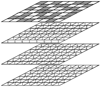
Multi-layer CA to generate normal random numbers |
As a result, the quality (randomness) of generated random numbers will be
decreased. Another approach to work out this issue is using linear or nonlinear
mappings. Clearly, if the length of primary range is bigger than the length
of desired range, odds of generating random numbers will differ.
To rectify this drawback, a different structure for cellular automata is presented in order to generate random numbers with normal distribution. The proposed structure possesses several distinct layers of CA. Each layer involves independent two dimensional cellular automata, all of the same size.
Cells of the first layer are binary which include only digits zero or one.
The goal is to generate normal random numbers in the range [0, n] and the pivot
is n/2, then the cells of second up to m(th) layer will include integer numbers
between zero and n. The structure of the proposed model is illustrated in Fig.
3. In first layer, each row encompasses independent linear binary cellular
automata. Therefore, each cell has two adjacent neighbors: one to the left and
one to the right. Associated values of cells in each row are updated using one
of the transition rules 30, 90, 105, 110 or 165.
A novel neighborhood structure named Pseudo Neumann is applied in other layers. In this model, similar to Moore standard neighborhood structure, for each cell, eight directly adjacent cells are considered as neighbors. The only way to distinguish Pseudo Neumann from Moore structure is that cells with the same positions from first layer with state equal to one are defined as active, otherwise they will be considered passive. If cells of the first layer generate uniform random bits, cells of other layers will be activate/passive with the same probability. In this sense, about half of the neighbors about four cells like Neumann structure will be active. Pseudo Neumann neighborhood structure is taken into account as Neumann neighborhood structure with dynamic adjacency due to the interaction between the first layer and other layers.
States of each cell in every layer excluding the first one is calculated as follows: at first, the sum of cell value and active neighbors values is computed; then the result is divided by n+1. Remainder of this division is the next value of cell. According to this rule, the values of cells will be between zero and n. Initial configuration of automata should be uniform. Whereby a finite number of values are equally likely to be observed; every one of values between 0 and n has equal probability 1/n. Now each cell in the second to m(th) layer is a uniformly distributed random number. To generate a normal random number, a cell is chosen from each layer (second to m(th) layer). Final normal random number is the mean of candidate cells values.
As stated in central limit theorem, since each cell in second to m(th) layer is an independent random variable, final result will be a random variable with normal distribution. If lower bound of needed random number is not zero, generated random number can be mapped to the desired range by using a simple linear transformation. If random number is in the range [-100,100], for example, n will be initialized with 200 and consequently output result will be in range of-100 to 100. In this method, number of layers affects standard deviation. In fact, according to central limit theorem, more layers will cause smaller standard deviation.
EXPERIMENTS AND RESULTS
In all experiments in this section, multi-layer cellular automata consisting
of a 1000x1000 cellular automata in each layer are used to generate normal random
numbers. Besides, the cells states in the first layer are updated by rule 30.
In the first experiment, the capability of binary cellular automata for producing
uniform random bits is examined. In second experiment, uniformity of generated
random numbers of proposed method is compared with random integer numbers generated
by MATLAB. In last experiment, quality (normality) of final results is assessed.
Experiment I: In this experiment, uniformity of generated random bits by linear cellular automata is evaluated. For this purpose, linear binary cellular automata possesses 100 cells. In this simulation, neighborhood radius is taken one and the rule 30 is used in order to change the cell states; 103 random bits were generated and total numbers of ones in the sequence were counted. This simulation had been executed 100 times and some significant statistical parameters such as mean, standard deviation and scattering length were calculated. The values of mean, standard deviation and scattering length for the numbers generated are 499.9484, 10.6328 and 86 accordingly which indicate that the quality of generated random bits using cellular automata is very desirable. In addition, the output random bits by cellular automata are uniformly distributed. Thus, it can be concluded that if rule 30 is used to update the values of first layer in the suggested model, the cells of other layers will be active or passive with approximately the same probability.
Experiment II: This experiment surveys the uniformity of random numbers generated by proposed model. To do so, at first a sequence of random numbers from a specific layer of the proposed model and random number generator of MATLAB are generated. Then, following steps are executed 100 times:
• |
Generate N = 104 random integer numbers in the
range of [0,100] |
• |
Classify the generated numbers in c = 10 classes with equal sizes |
• |
Compute the frequency of numbers in each class (fi) |
Finally, mean, standard deviation and scattering length of frequencies of numbers in each class are computed. Table 2 demonstrates experiment results.
From statistical perspectives, less standard deviation and scattering length
mean more uniformity. In other words, Table 2 reveals that
the distribution of generated random numbers by MATLAB is greater than output
of proposed multi-layer CA. Thus, it can be concluded that this method generates
more uniform numbers than MATLAB.
Table 2: |
Statistical parameters of experiment 2 |
 |
In the same way, mean indicator demonstrates that frequency of generated random
numbers (odds of being generated) in MATLAB random number generator is less
equal than proposed CA. In other words, it can be observed that proposed multi-layer
cellular automata generate more uniform random numbers with less scattering
length and standard deviation. It means that generated random numbers by proposed
cellular automata have equal probabilities.
Experiment III: On account of special characteristics of normal distribution,
investigating the normality of random numbers will be different. To evaluate
the normality, to date, many methods have been introduced (Ayanzadeh
et al., 2010), including:
• |
Kolmogorov-Smirnov test |
• |
Shapiro-Wilk test |
• |
Anderson-Darling test |
• |
Lilliefors test |
• |
Ryan-Joiner test |
• |
Normal probability plot |
• |
Jarque-Bera test |
• |
Spiegelhalter's omnibus test |
Most of these methods are experimental and based on empirical information.
Kolmogorov-Smirnov is widely known and discussed among all of above-mentioned
methods. The Kolmogorov-Smirnov test for normality is a nonparametric test which
can be applied to check whether data follow any specified distribution, not
just the normal distribution. In order to apply this test, sample cumulative
distribution and the hypothesized cumulative distribution should be computed.
Afterward, the greatest discrepancy between the observed and expected cumulative
distribution is found, which is called the "D-Statistic" (Ayanzadeh
et al., 2010; Lilliefors, 1967; Stephens,
1974). The Kolmogorov-Smirnov test is based on the Empirical Distribution
Function (ECDF). Given N ordered data points X1, X2,
,
XN, the ECDF is defined by Eq. 5:
where, n(i) is the number of points less than Xi. And Xi are ordered from smallest to largest value. Hypothesized distribution function FH(X) can be computed through Eq. 6:
|
Fig. 4: |
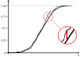
Maximum distance between distribution functions |
Where:
The maximum difference between the two distribution functions is computed and evaluated by Eq. 9:
Figure 4 is a plot of the empirical distribution function
with a normal cumulative distribution function. The K-S test is based on the
maximum distance between these two curves. In this figure, y axis specifies
the probability of random variable x or cumulative probability. In this experiment,
the maximum distance between numbers produced by MATLAB normal random number
generator and the ones produced by proposed multi-layer cellular automata are
calculated. FH(X) is assumed to be the desired normal probability
distribution function. Results for 102, 103, 104,
105 and 106 normal random numbers generated by proposed
model and MATLAB random number generator are shown in Table 3.
As can be seen from Table 3, the proposed multi-layer cellular
automata generate more normal results than MATLAB random number
generator. To be more precise, outputs of multi-layer cellular automata are
more similar to standard Gaussian distribution (with zero mean and unit variance)
than MATLAB normal random number generator.
Table 3: |
Statistical parameters of experiment 3 |
 |
From the perspective of statistics, probability distribution function of generated
random numbers by proposed CA has less distance with standard normal distribution
in comparison to MATLAB random number generator. Thus, generated random numbers
are more likely to be considered normal.
CONCLUSION
In this study, a unique method for generating high-quality normal random numbers is described in which multilayer cellular automata concept is employed along with Pseudo Neumann neighborhood structure. In this model, cells of automata which are responsible for producing random numbers contain integer values, contrary to previous methods in which random bits were generated using cellular automata. Binary cells in first layer are assumed to be active or passive by cells of binary automata; as a result, cellular automata obtained dynamic neighborhood structure.
The experiments were intended to assess the normality of random numbers generated from the proposed method. It was experimentally validated that multilayer cellular automata generate random numbers more normally distributed than random numbers generator of MATLAB. The main drawback for this method is improper initial configuration which may cause Garden of Eden. Different neighborhood structures and appropriate hardware implementation could improve the performance of multi-layer cellular automata model by applying hybrid transition rules.