
Wei Wei
School of Computer Science and Engineering, Xi�an University of Technology, Xi�an 710048, China
Bin Zhou
College of Science, Xi�an University of Science and Technology, Xi�an 710054, China
Information Technology Journal
Year: 2012 | Volume: 11 | Issue: 5 | Page No.: 632-636


ABSTRACT
A novel p-Laplace equation model is proposed in this paper for image denoising. First, the p-Dirichlet integral and total variation are combined to create a new energy functional used to built an image denoising model. This model is the generalization of Rudin-Osher-Fatemi model and Chambolle-Lions model. Then the existence of the solution can be obtained by the good properties of some functions in the nonlinear evolution equation. The numerical experiments with different parameters are implemented at last. The simulation results show the accuracy and efficiency of our method.
PDF Abstract XML References Citation
Received: November 21, 2011;
Accepted: January 04, 2012;
Published: February 22, 2012
How to cite this article
Wei Wei and Bin Zhou, 2012. A p-Laplace Equation Model for Image Denoising. Information Technology Journal, 11: 632-636.
DOI: 10.3923/itj.2012.632.636
URL: https://scialert.net/abstract/?doi=itj.2012.632.636
DOI: 10.3923/itj.2012.632.636
URL: https://scialert.net/abstract/?doi=itj.2012.632.636
INTRODUCTION
Generally, the practical images always hold the noise that does not only undermine the display but also affect the subsequent treatment results of the higher-level image. It is a big challenges to remove the noise of images with the maintainance of geometric characters during the scientific research and engineering practical activities. Therefore, denoising of image denoising is one of the important issues in the study of image processing and computer vision. Image denoising based on nonlinear diffusion equation is an effective method, about which many research achievements have been obtained and applied in many fields (Chan and Shen, 2005; Lysaker and Tai, 2006; Perona and Malik, 1990). The basic idea is to use different smooth policies at the target edge, namely at the edge area, the smooth process will be controlled but accelerated in the other regions.
Based on the nonlinear diffusion equation, the complex filtering process can be divided into two simple ones: one along the image gradient direction and the other perpendicular to the image gradient direction. The equations with better denoising results should have various diffusion rates in both directions, namely, diffusion process is anisotropics. This method can also retain the image geometry while removing the noise. There are some classic and anisotropics diffusion models. There are some classic and anisotropics diffusion models such as Perona-Malik model, mean curvature motion model, total variation model, among which total variation model (Rudin et al., 1992) give the following energy functional equation:
| (1) |
In the model, BV energy terms of the image Function model (based on the image gradient pattern energy term with L1 norm determined) determine the corresponding evolution equation that has a good non linear (has good non-linear) diffusion properties. In fact, the diffusion is unidirectional with non-zero diffusion velocity only in the tangent direction of horizontal lines of images which determines no demolishment of the important features of image structure but a certain effect of denoising during the evolution of the equation. However, in the local area of unimportant characteristics, the unidirectional diffusion speed becomes too slow and too single so as to affect the denoising effect and efficiency. If the energy term of I the equation s replaced by the L2 norm of the gradient mod, a thermal diffusion equation will be obtained which will cause excessive smoothing and loss of image features.
p-Laplace equation (Dibendetto, 1993), with a profound physical meaning, could be related to lots of natural phenomena. Until now, there are lots of theoretical achievements about p-Laplace equation. In this study, based on the total variation model, we firstly discuss the diffusion behaviors driven by p-Laplace which is applied to image denoising. A well-pose proof of the model is implemented with a discussion of numerical solutions. Finally, some related experimental results and conclusions are provided.
DIFFUSION BEHAVIORS DRIVEN BY p-LAPLACE
For the gray image function u(x): u(x): Ω⊂R2→R, analyzing the local anisotropic diffusion, as |∇u(x)|≠0, at the x point, we determined these two local directional vectors. In the gradient direction:
and the tangent direction:
then:
uN = |∇u|, uT = 0 |
subsequently computed and the following equation is obtained:
| (2) |
Consider the following energy term:
| (3) |
This is general p-Dirichlet calculus, the variation about υεC0∞(Ω):
| (4) |
From δEp = 0 and υεC0∞(Ω), p-Laplace equation is available:
| (5) |
It can be remarked as -Δpu = 0. In virtue of the direction vector N and T, p-Dirichlet calculus is rewritten as:
| (6) |
Theorem 1: Euler-Lagerange of Functional 6 is:
| (7) |
Proof: Whose proof is ignored.
An evolutive PDE is as follows in virtue of the gradient decline method:
| (8) |
When p = 2, this is equal to the heat equation. The diffusion term corresponds to the minimum energy term of the total variation model, namely when p→∞, ![]() corresponds to the infinite Laplace Δ∞u which can be defined as uNN (Aronsson et al., 2004) or u2NuNN (Oberman, 2005). Those were applied to the image fixing (Caselles et al., 1996) and the transforming problems (Cong et al., 2004).
corresponds to the infinite Laplace Δ∞u which can be defined as uNN (Aronsson et al., 2004) or u2NuNN (Oberman, 2005). Those were applied to the image fixing (Caselles et al., 1996) and the transforming problems (Cong et al., 2004).
MODEL OF IMAGE DENOISING BASED ON THE p-LAPLACE EQUATION
Chambolle and Lions use the heat diffusion term to accelerate the total variation model partially (Chambolle, 1995). Chen et al. (2006) studied the diffusion behaviours of variational exponentiate.
With the inspiration of these studies, this paper proposes the following function based on the p-Dirichlet Calculus and total variation of energy function:
| (9) |
where, u0 refers to the images that is needed to be denoised and the nonnegative function F(s) is defined as the following:
 |
Here, when β>0, p>1, F (s) is constant.
Set β = 2, p = 2.5 and Fig. 1 shows a comparison of the function F(s) and the function ![]() (heat diffusion model), the function f(s) = s (total variation model) when s is in smaller and bigger conditions.
(heat diffusion model), the function f(s) = s (total variation model) when s is in smaller and bigger conditions.
As is shown in the figures, with a smaller s, the value of function F(s) in this model decreases more quickly than that in the model of diffusion during the process of s→0; with a bigger value of s, it increases more slowly in the process of s→+∞. What is more, the increase in the value of the function F(s) in the model approaches that in total variation model which endows the evolutionary Eq. 8 minimized from the energy function with the expected diffusion attribute. When |Δu| is smaller, the diffusion will be accelerated but when |Δu| is larger, diffusion behaviors approach and then will be equal to that of the total variation model.
 | |
| Fig. 1(a-b): | Comparison F(s) of TV model and with that of heat diffusion model; (a) 0≤s≤β and (b) s>β |
The variation of E(u) is computed when υεC0∞(Ω):
| (10) |
When, δEp = 0, the evolution equation is obtained:
| (11) |
Where:
 | (12) |
From the above equation, as |∇u|≤β, the diffusion behaviors of Eq. 11 is driven by the term ∇. (|∇u|p-2Δu) of p-Laplace. If only |∇u|>1 and p>2 or |∇u|<1 and p<2, then the diffusion results show the exceeding effect of heat diffusion equation. When |∇u|>β behaviors of Eq. 11 is driven by the curvature term ![]() . Consequently, another form of evolutionary Eq. 11 is thus obtained.
. Consequently, another form of evolutionary Eq. 11 is thus obtained.
Theorem 2: The Eq. 11 is equal to the following form:
 | (13) |
Proof: The proof is ignored (Use the conclusion of Theorem 1).
Proof is ignored (Use the conclusion of theorem 1).
NUMERICAL EXPERIMENT
Utilizing the above mentioned model, we propose the preliminary boundary problem:
 | (14) |
where, the definition of:
is similar to that in Eq. 11. Through the adaptation of the method of Rudin et al. (1992), both sides of the first formula are multiplied by u-u0 and the integrations are also performed in Ω. Since t→∞, ![]() , then:
, then:
We can get the following after using the Green function:
Then it yields:
| (15) |
Here, the denominator ![]() dx is usually twice over noise variance which is usually predictable. After the numerical solution of the problem (14), the equation proposed in this study could be used in the field of denoising image.
dx is usually twice over noise variance which is usually predictable. After the numerical solution of the problem (14), the equation proposed in this study could be used in the field of denoising image.
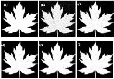 | |
| Fig. 2(a-f): | Results of transaction of phoenix tree leaves with noise; (a) Original image, (b) Noise image, (c) p = 1.0, (d) p = 1.6, (e) p = 2.0 and (f) p = 2.2 |
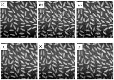 | |
| Fig. 3(a-f): | Results of rice-grains with noise; (a) Original image, (b) noise image, (c) p = 1.0, (d) p = 1.6, (e) p = 2.0 and (f) p = 2.2 |
As shown in Fig. 2a and b, given original images of phoenix tree leaves and denoised images, different p values are chosen to perform numerical solution which produces corresponding results.
Test 2.2: Figure 3a and b dividedly the original rice-grains images and denoising images. We utilize the proposed model to implement the denoising procedures with various p values.
Figure 2c-f and Fig. 3c-2f show the different results in the two experiments with various p-values. p-value, iterative numbers n of model solution, the solved results of Peak-signal-to-noise ratio (PSNR) are indicated in Table 1 and 2.
| Table 1: | P and n and PSNR data |
 | |
Given the constant p-value, with the iterative evolution, PSNR is gradually increased from values of 18.9763 and 18.7481 to the final results. The process is stable.
| Table 2: | Specific data of p, n and PSNR |
 | |
When, n is dramatically decreased by p-value, the PSNR value of final results is changed with a tiny visual effection. When, p = 1 and p = 2.0, the results are total variation model and Chambolle-lions model.
CONCLUSIONS
In this study, we utilize the p-Dirichlet calculus and TV energy to build p-Laplace equation model applied in the denoising process of images. The test results show that, according to the reasonably adjusting parameter p values, the presented model can dramatically decrease the iterative numbers with better denoising effects. It is very meaningful of vital significance for the issues of denoising in the complicated environment.
ACKNOWLEDGMENTS
We would like to thank the anonymous reviewers for their valuable comments. This study is supported by Scientific Research Program Funded by Shaanxi Provincial Education Department (Program No.11JK0504).
REFERENCES
- Aronsson, G., M.G. Crandall and P. Juutinen, 2004. A tour of the theory of absolutely minimizing functions. Bull. Am. Math. Soc., 41: 439-505.
Direct Link - Caselles, V., J.M. Morel and C. Sbert, 1996. An axiomatic approach to image interpolation. IEEE Trans. Image Process., 7: 376-386.
CrossRef - Chambolle, A., 1995. Image segmentation by variational methods: Mumford and shah functional and the discrete approximations. SIAM J. Applied Math., 55: 827-863.
Direct Link - Chen, Y., S. Levine and M. Rao, 2006. Variable exponent, linear growth functionals in image restoration. SIAM J. Applied Math., 66: 1383-1406.
Direct Link - Cong, G., M. Esser, B. Parvin and G. Bebis, 2004. Shape metamorphism using p-laplacian equation. Proc. 17th Int. Conf. Pattern Recogn., 4: 15-18.
Direct Link - Lysaker, M. and X.C. Tai, 2006. Iterative image restoration combining total variation minimization and a second-order functional. Int. J. Comput. Vision, 66: 5-18.
CrossRef - Oberman, A.M., 2005. A convergent difference scheme for the infinity laplacian: Construction of absolutely minimizing lipschitz extensions. Math. Comput., 74: 1217-1230.
Direct Link - Perona, P. and J. Malik, 1990. Scale-space and edge detection using anisotropic diffusion. IEEE Trans. Pattern Anal. Mach. Intell., 12: 629-639.
CrossRefDirect Link - Rudin, L.I., S. Osher and E. Fatemi, 1992. Nonlinear total variation based noise removal algorithms. Physica D Nonlinear Phenomena, 60: 259-268.
Direct Link