
Zhenyu Wu
Faculty of Electronic Information and Electrical Engineering, School of Innovation Experiment, Dalian University of Technology, Dalian 116024, People�s Republic of China
Yue Sun
Faculty of Electronic Information and Electrical Engineering, School of Innovation Experiment, Dalian University of Technology, Dalian 116024, People�s Republic of China
Bo Jin
Faculty of Electronic Information and Electrical Engineering, School of Innovation Experiment, Dalian University of Technology, Dalian 116024, People�s Republic of China
Lin Feng
Faculty of Electronic Information and Electrical Engineering, School of Innovation Experiment, Dalian University of Technology, Dalian 116024, People�s Republic of China
Information Technology Journal
Year: 2012 | Volume: 11 | Issue: 2 | Page No.: 217-224


ABSTRACT
Visual servoing referred to the technique which uses the computer vision data to control the motion of a robot. Among its various schemes, the image-based method was popular because of many advantages. But there were still some problems in its practical applications. Recently, a general control law of the image-based method using a behavior parameter had been proposed to improve the performance of the method. This study deals with the camera retreat problem and the image-based visual servoing scheme. The behavior-based visual servoing scheme was utilized. An analytical study of this scheme was presented when camera moves along and around the optical axis. The range of behavior parameter was obtained through the analytical study and rbf network. The camera retreat would not occur if the behavior parameter was picked in the range. When considering a difficult configuration, the study proposed an approach to adaptively select behavior parameter according to the range. Simulation results showed that this method compared with the classical image-base visual servoing schemes had better performance in avoiding the local minima in some configurations.
PDF Abstract XML References Citation
Received: September 17, 2011;
Accepted: October 25, 2011;
Published: December 31, 2011
How to cite this article
Zhenyu Wu, Yue Sun, Bo Jin and Lin Feng, 2012. An Approach to Identify Behavior Parameter in Image-based Visual Servo Control. Information Technology Journal, 11: 217-224.
DOI: 10.3923/itj.2012.217.224
URL: https://scialert.net/abstract/?doi=itj.2012.217.224
DOI: 10.3923/itj.2012.217.224
URL: https://scialert.net/abstract/?doi=itj.2012.217.224
INTRODUCTION
Visual servoing is a widely used method which can be applied to increase the accuracy, the versatility and the robustness of a vision-based robotic system. The goal of the visual servoing is to control the motion of a robot based on information extracted from the image of an object seen by a camera (Hutchinson et al., 1996; Hassanzadeh and Jabbari Asl, 2009). Three major schemes in the visual servoing control are image-based control (Espiau et al., 1992), position-based control (Wilson et al., 1996) and a hybrid approach (Malis et al., 1999). Among these schemes, the Image-based Visual Servoing (IBVS) is popular. This is because IBVS is robust and easy to implement when there are image noise and camera calibration errors. However, there are some difficulties in its practical applications. First, the control input and the error of image-based control approach are computed in two-dimensional image space. The approach does not estimate accurately enough the direction of displacement of the camera inducing unnecessary backward or forward motion (Chaumette, 1998). Second, using more than three feature points would require the use of pseudo-inverse or the transpose of the interaction matrix that introduce the risk of being trapped in a local minima (Chaumette, 1998; Lingfeng et al., 2002). Besides, image singularity may appear and the global asymptotic stability cannot be established even if the interaction matrix can be exactly computed (Chaumette and Hutchinson, 2006; Malis and Rives, 2003).
Much work has been done to improve the performance of IBVS in recent years. Allibert et al. (2010) proposed a predictive-control strategy which enables IBVS to take constraints into account easily. Tahri and Mezouar (2010) proposed a new appropriate formula of the ESM considering the tensor change of frames. Bai et al. (2009) proposed a control scheme based on fuzzy adaptive PID with a modified Smith predicator which resolved the problems of visual servoing’s inherent time delay. Zeng et al. (2008) proposed an improved broyden's method to estimate the image jacobian matrix on line which improves the effectiveness of visual servoing.
One of the major sources for the aforementioned issues originates from the interaction matrix. Marey and Chaumette (2008) analyzed three classical interaction matrix used in image-based visual servoing and proposed a behavior-based control law. The control law exploits the behavior parameter to adjust the weights of current and desired interaction matrix. The behavior of system shifts with the change of behavior parameter. In some configurations, this control law allows the robot to converge to the target position by picking the appropriate behavior parameter while all classical control schemes fail. Marey and Chaumette (2008) found the appropriate behavior parameters through experiments.
This study makes a further study of the above behavior-based visual servoing. The range of behavior parameter is obtained through the analysis of camera retreat problem and the study of camera motion along the optical axis. The camera retreat will not occur if the behavior parameter is picked in this range. This study also gives an approach to automatically select the behavior parameter according to the range.
MATERIALS AND METHODS
Effect of behavior parameter in motion along and around the optical axis: The study assumes the case of a motionless target and an eye-in-hand camera. Let sεR6 be the vector of the selected k visual features, s* their desired value and vεR6 the instantaneous velocity of the camera. Most classical control laws are given by:
| (1) |
where, λ is a gain and ![]() is the pseudo-inverse of an estimation or an approximation of the interaction matrix related to s (defined such that:
is the pseudo-inverse of an estimation or an approximation of the interaction matrix related to s (defined such that:
where, v = (υ, ω) with υ the translational velocity and ω the rotational one). Chaumette and Hutchinson (2006) summarized three different forms of ![]() :
:
| (2) |
| (3) |
| (4) |
Let Z be the distance between initial camera pose and target, Z* the distance between desired camera pose and target, θ the rotation of camera along the optical axis. Z and Z* are always greater than zero. Using different interaction matrix to control may induce retreat problem with different θ when Z and Z* (for example, Z>Z*) are given.
Applying Eq. 2 to control, the camera rotates and translates toward the desired pose without any additional movement as long as θ is less than an angle. When θ is greater than the angle, the camera continues its translation motion after reaching Z = Z* and then moves back toward the desired pose. The translation increases as θ increases. Due to this undesired translation the robot might reach the limit of its workspace.
Applying Eq. 3 (Malis, 2004) to control, the camera rotates and translates correctly as long as θ is less than an angle. When θ is greater than the angle, the camera starts moving backward and then translates forward. The translation increases as θ increases. Due to this undesired translation some features can go out of the camera field of view when the camera comes too close to the target.
Applying Eq. 4 to control, the camera moves without any supplementary translation as long as θ is less than 180. Marey and Chaumette (2008) give the general form of interaction matrix:
| (5) |
where, β is behavior parameter.
In order to study the impact of β on camera motion, the study firstly analyzes the case of motion along and around the optical axis. The task is to perform a translation of 0.5 m toward the target combined with a rotation of 120. A set of camera velocity curves is obtained with different β as shown in Fig. 1.
Figure 1 shows the velocity-time curves of camera motion. The translational velocity Vx, Vy and the rotational velocity Wx, Wy in the figure are always zero because the camera motion is along and around the optical axis (Z axis). There are no velocity components along X axis and Y axis. Negative values of translational Velocity curve (Vz) means that camera moves in opposite direction (back toward the target). The curve Vz in Fig. 1a indicates that camera starts moving backward and then translates toward the target. The curve Vz in Fig. 1f indicates that the camera continues its translation motion after reaching Z = Z* and then moves back to the desired pose. The camera can’t reach the desired position directly because of the existence of unnecessary translation. The camera moves forward normally in Fig. 1b-e because there are no negative values of translational velocity in the figures. The retreat problem just doesn’t appear in Fig. 1b and e. If β>0.628 or β<0.2857, the camera retreat problem will occur. Thus, there is a range of β that allows the camera to avoid retreat. Let βb be the upper limit of behavior parameter range and βa be the lower limit of behavior parameter range. A better performance of control system can be achieved if the selected β satisfies β∈(βa, βb). Approaches to obtain βa and βb will be given in the following sections.
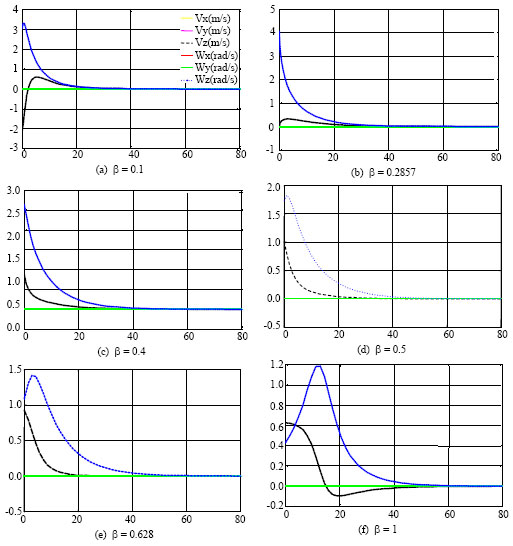 | |
| Fig. 1(a-f): | Camera velocity curves with different β when θ = 120° Z = 1 Z* = 0.5. There are only 3 trends in the figure because the translational velocity Vx, Vy and the rotational velocity Wx, Wy in the figure are always zero and overlap with each other. The camera motion is along and around the optical axis (Z axis). There are no velocity components along X axis and Y axis |
Approach to obtain βa: The camera displacement is a combination of a translation tz(from Z to Z*) and a rotation rz (rz = θ) with respect to the camera optical axis. The coordinates of a 3D point in the camera frame are denoted (X, Y, Z) and the coordinates of that point on the image plane are given by p = (x, y) with x = X/Z, y = Y/Z. The details of camera calibration and perspective projection can be found in many computer vision texts (Pu et al., 2011; Elatta et al., 2004; Arif et al., 2002). The interaction matrix related to p is given by:
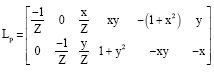 |
Using four feature points, the current visual vector is s = (x1, y1, x2, y2, x3, y3, x4, y4) and its desired value is s* = (x1*, y1*, x2*, y2*, x3*, y3*, x4*, y4*). The coordinates of the four points with respect to the camera frame at the initial and the desired poses are denoted Pi1 = (L, 0, Z), Pi2 = (0, -L, Z), Pi3 = (-L, 0, Z), Pi4 = wa 6 (0, L, Z) and Pd1 = (Lcosθ, Lsinθ, Z*), Pd2 = (Lsinθ, -Lcosθ, Z*), Pd3 = (-Lsinθ, -Lcosθ, Z*), Pd4 = (-Lsinθ, Lcosθ, Z*). The initial value of s is then si = (L/Z, 0, 0, -L/Z, -L/Z, 0, 0, L/Z). The desired value is s* = (Lcosθ/Z*, Lsinθ/Z*, Lsinθ/Z*, -Lcosθ/Z*, -Lcosθ/Z*, -Lsinθ/Z*, -Lsinθ/Z*, Lcosθ/Z*).
Applying the analytical form of Lp, it is possible to compute the analytical form of LG defined in Eq. 5:
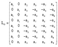 |
where, βε(0, 1):
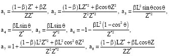 |
With the value of s - s*, the initial velocity v1 is easily deduced from Eq. 1 as:
v1 = (0, 0, υz, 0, 0, ωz) | (6) |
where, υz and ωz are the initial translational and rotational velocity of the camera:
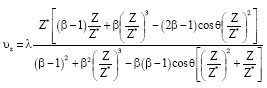 | (7) |
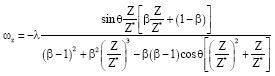 | (8) |
Equation 7 and 8 give a general form of vi which takes the effects caused by θ into account (Marey and Chaumette, 2008). According to the above experiment, the initial translational velocity of camera is zero when βa is used to control (Fig. 1b). Letting Eq. 7 be zero:
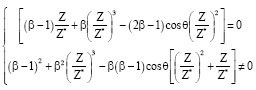 |
Through computations:
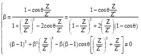 | (9) |
Equation 9 indicates that βa only relates to θ and Z/Z*. In order to verify Eq. 9, experiments are performed to get data points (βa) that should be satisfied by Eq. 9. Then, the study uses matlab sftool toolbox to fit the surface represented by Eq. 9 to experimental data. The βa under different θ and Z/Z* are shown in Fig. 2. The fit result is shown in Fig. 3. The goodness of fit is as follows: SSE 1.681x10⁻⁵, R/square 1, Adjusted R/square 1, RMSE 0.0003073. Figure 3 shows that all data points are exactly at the surface represented by Eq. 9. It can be seen from Fig. 2 that βa ε (0.5, 1) when the required motion is backward the target (Z/Z*<1) and βa ε (0, 0.5) when the required motion is forward the target (Z/Z*>1).
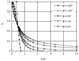 | |
| Fig. 2: | Experimental data for verifying Eq. 9 |
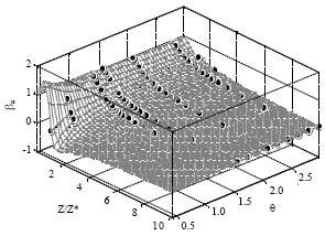 | |
| Fig. 3: | Fitting result |
Approach to obtain βb: Three factors that affect βb are θ, Z and Z*. Although the expression of βb is different from βa, βb and βa can both lead to the case that retreat just doesn’t appear. So the study assumes that the factor affecting βb is similar with that affecting βa, hence letting one factor of βb is Z/Z* and verifying the assumption with a set of experiments. θ is given by 120°, let Z be 0.5, 0.6, 0.7, 0.8, 0.9, 1 and the corresponding Z* 1, 1.2, 1.4, 1.6, 1.8, 2, respectively. The result in Table 1 shows that whatever the value of Z and Z* are, βb is constant as long as Z/Z* are same when θ is given. Thus, one factor affecting βb is Z/Z*.
It should be pointed out that the experiment is performed without limiting the camera velocity. The result change when the translational velocity is limited in -1.4, 1.4 (Table 2). In the first three cases, βb is as same as the one in Table 1. In the cases that Z/Z* are 0.8/1.6, 0.9/1.8 and 1/2, the camera velocity exceeds the limit during movement which leads to change in βb and it fails to meet our assumption. However, the retreat problem won’t occur if βb = 0.425 is used in the three cases. Therefore, it is meaningful to obtain βb without limiting the velocity and in this case βb only relates to Z/Z* and θ.
It is difficult to obtain the exact expression of βb with the aforementioned strategy when the initial translational velocity of camera has no obvious rule. One feasible method to find out the non-linear relationship among Z/Z*, θ, βb is approximating with numerous experimental data. In order to improve the approximation performance, the experimental data must be sufficient and have reasonable distribution. For example, θ can be picked every 10° from 30° to 170, Z/Z* can be picked from 0.1 to 10. The corresponding βb can be obtained by observing the camera translational velocity. Figure 4 shows the experimental data used for approximation. It can be seen that βb ε (0.5, 1) when the required motion is forward the target (Z/Z*>1) and βbε(0, 0.5) when the required motion is backward the target (Z/Z*<1).
Neural network has a strong non-linear fitting capability. RBF network has the advantages of fast learning, high accuracy and less chance of falling into local minimum (Kang and Jin, 2010; Qasem and Shamsuddin, 2010).
| Table 1: | Values of βb under the same Z/Z* |
| Table 2: | Values of βb under the same Z/Z* without limiting the velocity |
It can approximate nonlinear functions with arbitrary precision (El-Kouatly and Salman, 2008). Therefore, RBF network is used to approximate βb with experimental data. θ and Z/Z* need to be normalized before training the experimental data with new rb function of matlab neural network toolbox. It is important to ensure the spread parameter large enough to overlap regions of the input space but not so large that all the neurons respond in essentially the same manner. The spread parameter is given by 0.5 after tests. The mean square error of RBF network is about 9x10⁻⁷ after 300 steps of training as shown in Fig. 5a. In order to investigate the network response in more detail, postreg function is used to perform a regression analysis between the network response and the corresponding targets. As shown in Fig. 5b, it is difficult to distinguish the best linear fit line from the perfect fit line because the fit is good.
Approach to adaptively identify the behavior parameter: When the camera only moves along the optical axis, any value between βa and βb can be used to avoid camera retreat. When the camera displacement is large, not all values between βa and βb can be used to perform visual servoing task successfully. However, it is possible to utilize βa and βb to determine the value of β that provide a satisfactory behavior of the control scheme. The study chooses β = (βa+βb)/2. Thus, when Z, Z*and θ are given, β can be picked automatically according to Eq. 9 and the trained network. This method compared with classical schemes allows the system to avoid the local minima in some configurations.
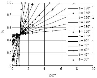 | |
| Fig. 4: | Approximation data of βb |
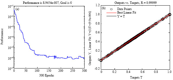 | |
| Fig. 5(a-b): | Training results |
RESULTS AND DISCUSSION
The study uses the matlab robotics toolbox and Simulink for the simulation. A pose is denoted as (t, r) where t is the translation expressed in meter and r is the roll, pitch and yaw angles expressed in radians. Four feature points are chosen as (0.1, 0.1, 0), (0.1, -0.1, 0), (-0.1, -0.1, 0), (-0.1, 0.1, 0). The initial camera pose and the desired camera pose in the world frame are chosen as (0.3 0.3 0.4 -0.7 0.5236 -1.0472), (-0.6 -0.6 0.8 0.7 -0.5 1.0472), respectively. In this case the image plane is not parallel to the target. The distance between the camera and the target is defined as the average of the four feature points’ depths. The simulation results obtained by using β = 0, β = 0.5, β = 1 and β = (βa+βb)/2 = 0.569 in the control scheme are shown in Fig. 6a-i. As can be seen, our method is the only one to converge to the desired pose.
Applying β = 1 in control scheme, the interaction matrix is constant and computed using the points depth at the desired camera pose (Espiau et al., 1992). In this case, the global asymptotic stability of the system will be achieved only in a smaller neighborhood. Some image features may leave the camera field of view during camera motion, particularly when the initial camera pose is far away from the desired pose (Lingfeng et al., 2002). In the experiment, due to the large displacement between the initial and the desired position, the camera starts to diverge so that the feature points get out of the camera field of view. The camera in this case can’t reach the desired position. The position error and the feature error become bigger with the passing of time (Fig. 6g-h).
Applying β = 0 in control scheme, the interaction matrix is updated at each iteration by the use of the estimated depth of feature points (Hutchinson et al., 1996). If the depth is exactly calculated, feature points in image plane will move to their desired positions in straight lines. It may imply inadequate camera motion in 3-D Cartesian space and lead to possible local minima (Chaumette and Hutchinson, 2006). In the experiment a local minima is reached when β = 0 is used since the camera velocity is zero while the final camera position is far away from its desired one (Fig. 6b). At that position the error s-s* in the image do not completely vanish (Fig. 6a).
Using β = 0.5 to control is a compromise between the two methods mentioned above (Malis, 2004; Tahri and Mezouar, 2010). The scheme fails in a local minima (Fig. 6e-d). Similar experimental results that exhibit the possible local minima problem of this scheme were obtained by Marey and Chaumette (2008) as well.
When β = 0.569 is used in the control scheme, the global minima is correctly reached from the same initial camera position and at the final camera position the image error disappears entirely (Fig. 6k-j). Chaumette (1998) pointed out that it is sometimes more interesting to use ![]() (β = 1) instead of
(β = 1) instead of ![]() (β = 0), because the control law using
(β = 0), because the control law using ![]() converge to a local minima while the use of
converge to a local minima while the use of ![]() allows to avoid this local minima in some configurations. Therefore, the system behavior will be better when the picked β is close enough to 1 but not so close that the feature points might leave the camera field of view.
allows to avoid this local minima in some configurations. Therefore, the system behavior will be better when the picked β is close enough to 1 but not so close that the feature points might leave the camera field of view.
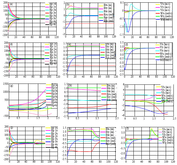 | |
| Fig. 6(a-l): | Experimental results: results using β = 0( (a) features errors (pixel) (b)camera pose error(c)camera velocity), results using β = 0.5( (d) features errors (pixel) (e)camera pose error (f) camera velocity), results using β = 1 ((g) features errors (pixel) (h) camera pose error (i) camera velocity), results using β = 0.569( (j) features errors (pixel) (k) camera pose error (l) camera velocity) |
CONCLUSION
The study utilizes a behavior-based visual servoing to study the camera retreat problem and identify the range of behavior parameter through analyzing the camera motion along the optical axis. For the lower limit of the range, an accurate expression is given. For the upper limit of the range, the study only finds out the relevant factors and approximates it by neural network. When the required motion is forward the target, the camera moves to the desired pose normally as long as the selected β satisfies βε(βa, βb). When the required motion is backward the target, βa is larger than βb, the camera moves to the desired pose normally when the picked β satisfies βε(βb, βa). An approach to automatically select behavior parameter is given when camera displacement is large. Future work will be devoted to find the exact expression of the upper limit of the behavior parameter and to the stability analysis of the method.
ACKNOWLEDGMENT
This study is supported by National Natural Science Foundation of People’s Republic of China (Grant No. 61173163, 51105052), Program for New Century Excellent Talents in University (Grant No. NCET-09-0251) and Liaoning Provincial Natural Science Foundation of China (Grant No. 201102037).
REFERENCES
- Chaumette, F. and S. Hutchinson, 2006. Visual servoing control. I. Basic approaches. IEEE Robot. Autom. Mag., 13: 82-90.
CrossRef - Espiau, B., F. Chaumette and P. Rives, 1992. A new approach to visual servoing in robotics. IEEE Trans. Robot. Autom., 8: 313-326.
CrossRef - Hutchinson, S., G.D. Hager and P.I. Corke, 1996. A tutorial on visual servo control. IEEE Trans. Robot. Automat., 12: 651-670.
CrossRefDirect Link - Malis, E., F. Chaumette and S. Boudet, 1999. 2-1/2-D Visual Servoing. IEEE Trans. Robot. Autom., 15: 238-250.
CrossRefDirect Link - Malis, E., 2004. Improving vision-based control using efficient second-order minimization techniques. IEEE Int. Conf. Robot. Autom., 2: 1843-1848.
CrossRef - Marey, M. and F. Chaumette, 2008. Analysis of classical and new visual servoing control laws. Proceeding of the International Conference of Robotics and Automation, March 19-23, 2008, Pasadena, CA., USA., pp: 3244-3249.
CrossRef - Wilson, W.J., C.C.W. Hulls and G.S. Bell, 1996. Relative end-effector control using cartesian position based visual servoing. IEEE Trans. Robot. Autom., 12: 684-696.
CrossRef - Tahri, O. and Y. Mezouar, 2010. On visual servoing based on efficient second order minimization. Rob. Auton. Syst., 58: 712-719.
CrossRefDirect Link - Allibert, G., E. Courtial and F. Chaumette, 2010. Predictive control for constrained image-based visual servoing. IEEE Trans. Rob., 26: 933-939.
CrossRefDirect Link - Hassanzadeh, I. and H. Jabbari Asl, 2009. Tele-visual servoing of robotic mamipulators: Design, implementation and technical issues. J. Applied Sci., 9: 278-286.
CrossRefDirect Link - Bai, L., F. Chen and X. Zeng, 2009. Fuzzy adaptive proportional integral and differential with modified smith predictor for micro assembly visual servoing. Inform. Technol. J., 8: 195-201.
CrossRefDirect Link - Zeng, X., X. Huang and M. Wang, 2008. Micro-assembly of micro parts using uncalibrated microscopes visual servoing method. Inform. Technol. J., 7: 497-502.
CrossRefDirect Link - Kang, P. and Z. Jin, 2010. Neural network sliding mode based current decoupled control for induction motor drive. Inform. Technol. J., 9: 1440-1448.
CrossRefDirect Link - Qasem, S.N. and S.M. Shamsuddin, 2010. Generalization improvement of radial basis function network based on multi-objective particle swarm optimization. J. Artif. Intell., 3: 1-16.
CrossRefDirect Link - El-Kouatly, R. and G.A. Salman, 2008. A radial basic function with multiple input and multiple output neural network to control a non-linear plant of unknown dynamics. Inform. Technol. J., 7: 430-439.
CrossRefDirect Link - Pu, Y.R., S.H. Lee and C.L. Kuo, 2011. Calibration of the camera used in a questionnaire input system by computer vision. Inform. Technol. J., 10: 1717-1724.
CrossRef - Elatta, A.Y., L.P. Gen, F.L. Zhi, Y. Daoyuan and L. Fei, 2004. An overview of robot calibration. Inform. Technol. J., 3: 74-78.
CrossRefDirect Link - Arif, M., H. Xinhan and W. Min, 2002. Stratified approach to 3D reconstruction. Inform. Technol. J., 1: 75-79.
CrossRefDirect Link