An Optimal Control Model and the Computer Algorithm for the Diffusion Parameter of the Drug Releasing in the Spherical Device

INTRODUCTION

The optimal control models and the computer methods for designing the delivery devices of the drug releasing have been paid attention in the recent years (Mwellott et al., 2001; Siepmann et al., 1998; Hukka, 1999; El-Sersy, 2007; Parra-Guevara and Skiba, 2003). In order to design the drug delivery system, it is important to compute the diffusivity and the diffusion process in some special delivery systems. For this reason, many computational methods and the computer software are used to compute the effective diffusion process (Arunachalam and Annadurai, 2011; Hefny, 2007; Rao et al., 2011; Kossah et al., 2010). However, many computation methods and the optimal models depended on the special cases in 2D or on the empirical model and the linear problems. (Zhu and Zeng, 2002; Kohne et al., 2002; Grassi and Grassi, 2005; Thomes, 1995). For the special materials, many optimal models for designing the delivery devices are nonlinear and complicated. (Singh et al., 2011; Dash and Gummadi, 2007). Computing the nonlinear optimal model and the complicated linear optimal model becomes one cost-time problem. Therefore, it is necessary to find out the computing method to save the computing time for dealing with the special cases or the 3D cases (Grassi and Grassi, 2005; Lee et al., 1999; Balamuralidhara et al., 2011).

In previous papers (Li et al., 2010, 2011), in order to be better to analyze the 3D cases than before, we proposed a numerical method to extract the diffusion coefficients from the diffusion and convection-diffusion processes. However, in fact, for the numerical method, it cost too much time to obtain the best approximation of the mass rate because the numerical method computing the releasing rate of the drug had many numerical equations simulating the diffusion process. For these reasons, in this study, we proposed a new computer optimal model and the optimal computer method based on the Least Square Method and the Separation of Variables (LSMSV) to extract the diffusion coefficients from the diffusion processes in the sphere device.

THE OPTIMAL CONTROL MODEL TO COMPUTE THE DIFFUSION PARAMETER IN THE SPHERE DEVICE

The optimal control problems governed by the diffusion equations arise in many scientific and engineering applications, such as the atmospheric pollution control problems and the drug releasing fields. This study is devoted to solving the following diffusion equation in the sphere device:

(1)

where, D is the diffusion constant parameter and C (x, y, z, t) is the drug concentration.

For the initial condition H (x, y, z), we assume that at t = 0, the drug concentration is uniform in the device and zero in liquid i.e.:

(2)

The domain is the sphere device as Fig. 1 including the black sphere domain Ω₁ that includes the diffusion material and the white sphere domain Ω that includes the liquids.

The following process is to use the spherical polar coordinate system to replace the Eq. 1. The spherical polar coordinate is:

(3)

Substituting (3) in (1), we can obtain:

(4)

Owing to the sphere being symmetrical, the concentration C = C (r, t) is independent of θ and φ in the sphere device. The Eq. 4 can be written as:

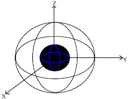Fig. 1:	Drug delivery device including the black sphere Ω1 and the white sphere Ω

(5)

Using:

and setting u = rC, we have:

The boundary condition in Eq. 1 can be translated into:

(6)

For:

the initial condition (6) can be translated into:

So, the three-dimensional diffusion Eq. 1 in the sphere device can be changed into the one-dimensional diffusion Eq. 7:

(7)

where, u = rC.

In order to obtain the diffusion concentration in the sphere device, it is necessary to divide the radius interval [R₁, R₂] into many enough short sections. Set R₁ = r₁<r₂<...<r_k = R₂, we can get the diffusion concentration of each radius intervals [r₁, r₂], [r₂, r₃], ... , [r_k-1, r_k]. From the concentration in the same time, the mass M_i1, ..., M_{i (k-1)} in each section denoting the mid-value of the drug concentration in each radius interval. Therefore we can get the total mass M_i = M_i1+ ... +M_{i (k-1)} in [R₁, R₂].The idea is induced as following:

Problem 1: Find D to satisfy the:

(8)

where, M₁⁰, M₂⁰, ..., M_e⁰ are given experimental data and M₁, M₂, ..., M_e are computed by the following formula:

and:

(9)

THE SEPARATION OF VARIABLES METHOD BASED ON DRUG RELEASING IN SPHERE DEVICE

In the following section, based on the separation of variables method (Thomes, 1995) to solve the Eq. 7, we can get the solution of the Eq. 7:

(10)

where, β_n(n = 1, 2, ...) is the positive root of tanx = x and E_i (i = 0, 1, 2, ...) are the expand coefficients, in the following section, we shall decide these expand coefficient E_i (i = 0, 1, 2, ...).

When t = 0 with the initial condition, there is:

(11)

To choose the coefficient to satisfy:

(12)

Multiple r², then integration from r = 0 to r = R₂, we can get:

For Eq. 12:

Because:

is always true, we can obtain:

Both sides of Eq. 11 multiple:

then integration from r = 0 to r = R₂, the following equation can be got:

By Eq. 12, there is:

and:

If m≠n, then:

and:

where, the coefficient is:

Therefore, the concentration can be computed as follows:

(13)

For the derivative C’ (r, 0) of the piecewise continuous function and C (r, 0) is piecewise function, C (r, 0) is a piecewise smooth function. By the Fourier series convergence theorem, the Fourier series of (13) is convergence to:

(1)	C (r, 0) (C (r, 0) at the continuous point)
(2)	(R1 is the discontinuous point of C (r, 0)

So:

(14)

where, β_n (n = 1, 2, ...) is the positive root of tanx = x.

LEAST SQUARE METHOD FOR SOLVING THE OPTIMAL CONTROL PROBLEM

Let:

(15)

where, M = (M1 (D), M2 (D))^T and M* = (M₁⁰, M₂⁰, ..., M_e⁰)^T.

We now consider the optimal numerical solution of the Problem 1. For an initial diffusion parameter point D⁰, Problem 1 can be solved iteratively by the following deduction. An increment δDⁱ in each step is calculated as follows:

Minimizing E (Dⁱ+δDⁱ) with respect to δDⁱ, where Dⁱ and δDⁱ are the ith approximation and ith increment of D, respectively.

Let:

So

(16)

The Eq. 15 can be written as follows:

(17)

For f_i (D) are the nonlinear functions, (16) is a nonlinear least square problem. To solve this problem, we can use the linear least square method to solve the nonlinear least square problem. Suppose that D_(k) be the kth approximation and let the function f_i (D) to be the linear function at D_(k), the minimal point D_(k+1) and the (k+1)th approximation can be computed by the iterative method. The iterative formula is deduced in details as follow. Set:

The first term in the right hand of the above equations are the first order Taylor expansion polynomials at D_(k) and set:

(18)

Use φ(D) to replace F (D) and use the minimal point of φ(D) to estimate the function F (D). Next, to solve the least square problem: φ(D), set:

(19)

(20)

So, Eq. 18 can be written as:

In order to search the stable point of φ(D), set

(21)

taking A and B into (21), the following equation can be obtained:

Moving A^T AD_(k) to the left hand in the above equation, there is

(22)

Obviously, this is a linear equation depending on the function value and first order partial derivative f_i (D_(k)) at the point D_(k), if the matrix A is the full column rank, A^T A is a symmetry positive matrix. Therefore, there is (A^TA)^-1, we can get the stable point of the Eq. 22 as:

follows:

(23)

By the above deduced formula, the optimal algorithm based on the least square method based on the separation variables method (LSMSV) extracting the diffusion parameters are represented as follows step by step.

Algorithm (LSMSV) :

NUMERICAL EXAMPLE

In order to test the convergence, the computing velocity and the validity of the proposed scheme, an example is given in this section. The spherical device is divided into large and small spherical structures where small spherical container including the drug is fixed in the large and the large container is filled with the liquid. The radius of small and large sphere devices are 0.4800 and 2.8399 dm, respectively and there is 500 g of drug in small spherical vessel. When t = 0, the inner concentration is 1079.33855, the outer is 0. After some diffusion process in a period of time, suppose time is 1079.33855, the inner and outer concentration is equal and is 5.2116, it is:

Set the following formula compute the total error in order to estimate the convergence rate:

We firstly compute the diffusion process to obtain the experiment data of the concentration shown in Table 1 according to the given diffusion parameter D = 0.0006. Next, using the above optimal computer algorithm (LSMSV) to estimate the diffusion parameter based on the optimal control model of the drug releasing in the sphere device and the mass.

Suppose the time interval be 60 sec and get 18 terms in Bessel function, by the LSMSV algorithm, the optimum points and their error values in each optimal step are given in the Table 2. In order to illustrate the convergence of the LSMSV algorithm, the optimal increment δD and the optimal values D of the diffusion parameter are depicted as Fig. 2 and 3.

In order to illustrate the convergence of the algorithm (LSMSV), we discuss the convergence data as follows: from the second column in Table 2 and Fig. 3, the increments δD convergent are very fast because their values become from 1.3867x10^-4 to 7.6555x10^-7. From the last column in Table 2, the optimized value D also becomes very fast from 2.3867x10^-4-6.0000x10^-4 by only six iterated times.

Table 1:	The change of drug quality

Fig. 2:	The error value of the optimized diffusion parameters by (LSMSV)

Fig. 3:	The increment of the optimized diffusion parameters by (LSMSV)

Fig. 4:	The optimized diffusion parameters by the algorithm (LSMSV)

Therefore, from the analysis in Table 2 and Fig. 2 and the error value in Fig. 3, the data show the error and the increment δD convergent stately. It is easy to illustrate the convergence of the algorithm (LSMSV).

In order to test the convergent velocity, we obtain the computing time to compute the optimal parameters by the algorithm (LSMSV) in the numerical examples. The computing time is less than one hour by the algorithm (LSMSV) in this example. In order to test the merits of the LSMSV algorithm, it is hard for us to use the algorithm in the study (Li et al., 2010, 2011) to compute the parameter values. However, the idea of LSCA for the sphere and the 3D disc in the study (Li et al., 2010, 2011) is same. Therefore, we use the computing time of LSMSV for the sphere domain to compare the computing time of LSCA for the disc in 3D.

The computing time shows that the LSMSV algorithm to compute the 3D sphere is very faster than the algorithm to compute the 3D discs in the paper (Li et al., 2010, 2011) because the LSCA algorithm to compute the optimal value costs more than one week.

Fig. 5:	Comparing the diffusion mass computed and the experimental data

Table 2:	The error value, the increment of the optimized diffusion parameters and the optimal diffusion parameters based on the initial value 0.0001

In addition, from the computing processes, it is also easy to understand why the computing velocity become very high because the algorithm in this paper only compute some the polynomial functions in each iteration to cost only less than 10 minutes, however , the algorithm in (Li et al., 2010, 2011) needs computing millions linear equations in each iteration to cost more than one day. Therefore, from the computing convergent time and in the computational theory, we can obtain the conclusion that the convergent velocity of algorithm (LSMSV) is very fast.

In order to estimate the validity of the algorithm (LSMSV), the error values between the experiment values and the computed values by the LSMSV algorithm are shown in Fig. 4 and the first column in Table 2, the optimal computed drug mass depending on the different optimal diffusion parameters and the experiment mass are depicted in Fig. 5. From the first column in Table 2, the errors of the optimized value D and the parameters is only 0.00003x10^-4, the error between the optimal computed drug mass 473.2175 g and the experiment mass data 486.1531 g is only 12.9356 g and the relative error of the mass is only 2.6%. The error result shows the algorithm (LSMSV) is valid to extract the diffusion parameter of the drug releasing in the sphere devices. From the numerical example, comparing the data of all iterative steps of the optimization values and the experimental data, it is easy to get the conclusion that the algorithm (LSMSV) is the convergent, fast and effective algorithm to extract the diffusion parameters of the drug releasing in the sphere devices.

REFERENCES

- Siepmann, J., A. Ainaoui, J.M. Vergnaud and R. Bodmeier, 1998. Calculaiton of the dimensions of drug polymer devices based on diffusion parameters. J. Pharm. Sci., 87: 827-832.
CrossRefDirect Link - Hukka, A., 1999. The effective diffusion coefficient and mass transfer coefficient of nordic softwoods as calculated from direct drying experiments. Holzforschung, 53: 534-540.
Direct Link - El-Sersy, N.A., 2007. Bioremediation of methylene blue by Bacillus thuringiensis 4 G1: Application of statistical designs and surface plots for optimization. Biotechnology, 6: 34-39.
CrossRefDirect Link - Parra-Guevara, D. and Y.N. Skiba, 2003. Elements of the mathematical modeling in control of pollutants emissions. Ecol. Model., 167: 263-275.
CrossRef - Arunachalam, R. and G. Annadurai, 2011. Optimized response surface methodology for adsorption of dyestuff from aqueous solution. J. Environ. Sci. Technol., 4: 65-72.
CrossRefDirect Link - Hefny, M.M., 2007. Estimation of quantitative genetic parameters for nitrogen use efficiency in Maize under two nitrogen rates. Int. J. Plant Breed. Genet., 1: 54-66.
CrossRefDirect Link - Rao, T.P., K.S. Rao and C.L. Usha, 2011. Stochastic modeling of blood glucose levels in type-2 diabetes mellitus. Asian J. Math. Stat., 4: 56-65.
CrossRefDirect Link - Kossah, R., C. Nsabimana, H. Zhang and W. Chen, 2010. Optimization of extraction of polyphenols from syrian sumac (Rhus coriaria L.) and chinese sumac (Rhus typhina L.) fruits. Res. J. Phytochem., 4: 146-153.
CrossRefDirect Link - Kohne, J.M., H.H. Gerke and S. Kohne, 2002. Effective diffusion coefficieents of soil aggregates with surface skins. Soil Sci. Soc. Am. J., 66: 1430-1438.
Direct Link - Grassi, M. and G. Grassi, 2005. Mathematical modelling and controlled drug delivery: Matrix systems. Curr. Drug Deliv., 2: 97-116.
Direct Link - Singh, M.R., D. Singh and S. Saraf, 2011. Formulation optimization of controlled delivery system for antihypertensive peptide using response surface methodology. Am. J. Drug Discovery Dev., 1: 174-187.
CrossRef - Dash, S.S. and S.N. Gummadi, 2007. Optimization of physical parameters for biodegradation of caffeine by Pseudomonas sp.: A statistical approach. Am. J. Food Technol., 2: 21-29.
CrossRefDirect Link - Lee, W.R., S. Wang and K.L. Teo, 1999. An optimization approach to a finite dimensional parameter estimation problem in semiconductor device design. J. Comput. Phys., 156: 241-256.
Direct Link - Balamuralidhara, V., T.M. Pramodkumar, N. Srujana, M.P. Venkatesh, N.V. Gupta, K.L. Krishna and H.V. Gangadharappa, 2011. pH sensitive drug delivery systems: A review. Am. J. Drug Discovery Dev., 1: 24-48.
CrossRefDirect Link - Li, Y., Z. Xiang, X. Xiang and S. Wang, 2010. A computer algorithm for optimizing to extract effective diffusion coefficients of drug delivery from cylinders. Inform. Technol. J., 9: 1647-1652.
CrossRefDirect Link