
M. H. Saheb
Department of Information Technology, Administrative Sciences and Informatics College, Palestine Polytechnic University, Palestine
Information Technology Journal
Year: 2011 | Volume: 10 | Issue: 1 | Page No.: 201-206


ABSTRACT
This study introduces Overlap-Join which is non-equi self join that joins a table to itself with a non-equal condition for joining. Overlap-Join arises in real word queries that deal with time. Time scheduling and time tabling applications are clear examples for time overlapping, this in addition to its usage in temporal databases. JOIN is the most expensive operation in relational databases. For this reason an efficient algorithm is needed. Overlap-Join and two parameters for Overlapping; Overlap Coefficient (OC) and Span Coefficient (SC) have been defined. Three properties for overlapping has been developed and discussed. Two algorithms have been proposed. These algorithms are modified versions of two known join algorithms; the block nested-loop join and the Sort-merge join. Models for joining costs have been presented and analyzed. The modifications take advantage of the fact that overlap-Join is self-join and the sc concept. The study shows that performance of sort-merge join is not better than the performance of block nested loop join for Overlap-Join when the SC is high.
PDF Abstract XML References Citation
Received: May 02, 2010;
Accepted: July 20, 2010;
Published: October 19, 2010
How to cite this article
M. H. Saheb, 2011. Efficient Algorithm for Overlap-Join. Information Technology Journal, 10: 201-206.
DOI: 10.3923/itj.2011.201.206
URL: https://scialert.net/abstract/?doi=itj.2011.201.206
DOI: 10.3923/itj.2011.201.206
URL: https://scialert.net/abstract/?doi=itj.2011.201.206
INTRODUCTION
An SQL JOIN clause combines tuples from two tables to produce the joined table. Join operations and Cartesian product are the most expensive operations frequently occurring in a database system (Noh and Gadia, 2008). So, all query optimization algorithms primarily deal with joins (Sinha and Chande, 2010). Join operation is more critical in temporal databases (Gao et al., 2005). During the last three decades many approaches have been developed for processing join operations efficiently. For a survey see Graefe (1993) and Soo et al. (1994).
There are many types of join; they include inner join and outer join. Equi-join and non-equi-join are types of inner join. Joining table to it is called self-join. Overlap-join is a class of non-equi self join.
There are many join algorithms for joining. However, they focus on joining different inputs rather than an identical input leading to multiple scans for the identical input (Noh and Gadia, 2005).
Overlap-Join arises in real word queries that deal with time. Time scheduling and time tabling applications are clear examples of time overlapping. Time overlapping is not allowed in scheduling problems, such as Airport runway assignment (Saffarzadeh et al., 2008). This in addition to its usage in temporal databases.
Here, we will concentrate on reviewing related works to Overlap-Join and not the general join operations. Many methodologies for join operations can be found in literature (Noh and Gadia, 2005, 2008). Gao et al. (2005) summarized join operations in temporal databases to include nested-loop join, sort-merge join and partition-based join.
Join operation in the temporal database literature is more concentrated on join operations for heterogeneous relations rather than self-join.
Range join, band join and bound join are special case of non equi-join. De Witt et al. (1991) presented algorithm for Band join. Band join is a class of non-equijoins. A band join between relations R and S on attributes R.A and S.B is a join in which the join condition can be written as R.A-C1≤ S. B≤R. A + c2. The constants c1 and c2 may equal and one of the two may be zero. We use the term band because a tuple r in R joins with a tuple s in S only if r.A appears within a Band of size c1 + c2 about s.B.
Shen (1995) presented an algorithm for Range join. Range join of sets R and S is defined to be the set containing all tuples (r, s) that satisfy e1 ≤ |r - s| ≤ e2 where r∈ R, s ∈ S, e1 and e2 are fixed constants.
Band joins and range join is not self join, while overlap-join is self join. Band and range are fixed, but overlap has variable ranges depending on the start and the end in each tuple as we will see in the definition of the overlap-join. So, general join algorithms cannot be used directly and they are not efficient.
Overlap-join definition: Join operation is a binary operator in relational algebra. It is written as (R![]() Φ S) where R and S are relations and theta is a condition for joining. The result of Join is a relation that contains all the
Φ S) where R and S are relations and theta is a condition for joining. The result of Join is a relation that contains all the
combinations of tuples in R and S that satisfy theta. If the condition in theta is = operator, then we call it equi-join, if not, then we call it non equi-join. If R and S are the same relation then the join is self-join (Elmasri and Navathe, 2007).
Overlap-Join is a class of non-equi self join. Assume that we have a relation:
where, a1 is the primary key, as attribute represents start time and ae attribute represents the end time, the overlap-join is: self join of R where (R.as between R'.as and R'.ae) and R.a1 < > R'.a1
We can represent this join using the following SQL SELECT statement syntax:
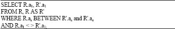 |
The FROM clause produce Cartesian product of R to itself. The first condition in WHERE clause converts the Cartesian product to JOIN by joining each row of R with any row of R such that the start (as) between any start and end (R'.as and R'.ae) in any row in R. The second condition prevents joining any row to itself, assuming that R.a1 is a candidate key.
Overlapping Coefficient (OC), defined as the average density of overlapping, used as a measure of overlapping of each tuple in the relations with other tuples in the same relation.
Overlap occurs in the following cases assuming that P is a period starts at s and ends at e:
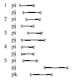 |
From these cases we can see that the following properties are hold for overlapping:
| • | Reflexive: If pi⊆pj, then pi overlaps with pj (Schikuta, 2003; PostgreSQL, 2002) |
| • | commutative property: If pi OVERLAP pj, then pj OVERLAP pi |
| • | If P is set of ordered periods sorted on p.s, such that pi.s ≤ pj.s for all i<j then pi will not overlap with any period after pj if pi.e<pj.s |
Span overlapping occurs when a tuple overlaps with more than one tuple and these tuples have no overlapping as in case 5. Spanning can occurs between blocks of tuples. We will define Span Coefficient (SC) as the average of overlapping of tubles in a block with the tuples in previous or next blocks. If SC = 1, then in average the tuples in any block overlapped with tubles from one block surrounding that block. If SC = n then, in average, the tuples in the current block can overlap with any tuple in the next n blocks or n previous blocks.
Overlap-join in SQL: We can define a hypothetical SELECT statement to address this overlap join. A simple BNF for this statement can be expressed as follows:
The optional part of this statement means that there is an Overlap join for the Relation R on the two attributes A1 and A2.
Postgre SQL (PostgreSQL, 2002) supports: OVERLAPS operator:
| • | (start1, end1) OVERLAPS (start2, end2) |
| • | (start1, length1) OVERLAPS (start2, length2) |
This expression yields true when two time periods (defined by their endpoints) overlap, false when they do not overlap. The endpoints can be specified as pairs of dates, times, or time stamps; or as a date, time, or time stamp followed by an interval. This is an operator and it is not used for JOIN operation.
ALGORITHMS FOR OVERLAP-JOIN
Many approaches can be used for joining operation; the following are the most popular approaches:
| • | Nested loop Join |
| • | Block Nested Loop Join |
| • | Partitioned based join |
| • | Sort-merge based join |
| • | Hash Join |
The last three algorithms cannot be used directly since these algorithms are for equi-join and Overlap-join is non equi-join. The first two algorithms can be used with some modifications, but all these algorithms will not work efficiently since they do not take advantage of the fact that this is self-join.
| Table 1: | Models parameters and derived terms |
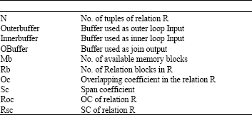 | |
Three algorithms and performance model will now be presented and discussed.
Access complexity: Here, we discuss the access complexity of the proposed modified algorithms. We will discuss the disk input complexity rather than I/O complexity. Output operation will not be included since it depends on the Roc and the Rsc of the overlapping. Table 1 defines some notations to be used in our analysis. It is clear that the size of the relation and the buffer size will have the major effect on the derived complexity.
In Table 1 we specify several parameters and a few derived terms which describe the characteristics of the model environment and build the basis for the derived cost functions.
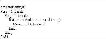
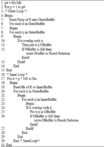
Nested loop join: Algorithm 1 represents nested loop join, it is a brute force join and each tuple in relation R is checked for possible join with all other tuples in R.
It is clear that the access complexity (Input Complexity) of this algorithm is O(n2).
| Algorithm 1: | Naïve algorithm (nested loop algorithm) |
 | |
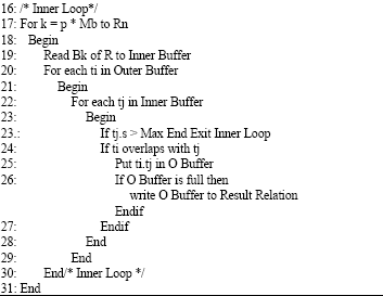
Modified block nested loop join: This algorithm starts by reading the first partition of R in the main Outerbuffer, each partition of the relation R consists of Mb blocks. Each tuple in the Outer buffer is checked for overlapping with all the other tuples in Outer buffer. For each overlapped tuples we put the joined tuples in Obuffer we check if the OBuffer is full, we write it to the result realtion. The second stage; marked as inner loop in Algorithm 2, starts by reading each block of R after the last block which was loaded in the outerbuffer and putting it in the innerbuffer. Then each tuple in the outerbuffer is checked for overlapping with all the tuples in innerbuffer. For each overlapped tuples we put the joined tuples in Obuffer checking if the Obuffer is full, we write it to the Result relation. This process will be repeated for each partition of the relation R. Figure 1 represents the first loop of the outer loop.
Block nested-loop join complexity: The complexity (I/O Complexity) of this algorithm is composed of two parts; the number of input blocks and the number of output blocks from OBuffer to the Result relation.
The number of input blocks includes:
| • | Reading all the blocks in R; Mb block each loop of the outer loop = Rb |
| • | Reading the blocks after the partition which is in the outerbuffer |
| Algorithm 2: | Modified block nested loop join |
 | |
 |
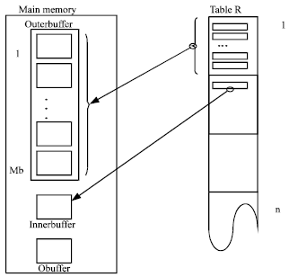 | |
| Fig. 1: | First loop in the block nested loop join |
where, p is the number of partitions (Rb/Mb). So, the complexity of blocks readings is :
The number of blocks to be written depends on the Overlapping Coefficient (OC) in the relation.
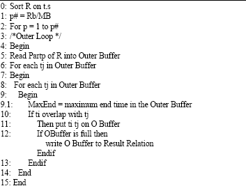
Modified sort-merge based join: The conventional sort-merge based join algorithm is used for equi-join of two relations; R and S. It starts by sorting the two relations on the joining attribute in each relation. As first stage, we can use an external sorting algorithm. The second stage merges the two relations on joining condition. This method of joining works very well for equi-join since all participating tuples in joining each relation are sequenced.
| Algorithm 3: | Modified sort-merge join algorithm |
 | |
 | |
The joined tuples in overlap-join will be scattered in the sorted relation, the joining algorithm will be in general the same algorithm for Nested Block join. We will take advantage from the sorting and property-3 of overlapping properties, this means no tuple can overlap with all the tuples that started after the end of that tuple. Tuples in R are sorted on the start time.
Algorithm 3 is a modified version of Algorithm 2. Three lines has been added; line-0 sorts the relation R on the start time, line 9.1 finds the maximum end time for all tuples in Outer Buffer to be used for limiting the search for overlapping tuples in line 23.1.
Modified sort-merge bases join complexity: A sort-Merge base join algorithm always performs better than Nested-Block join algorithms for equi-join. This is clear in the literature of joining operation. But as we will see in our analysis of Overlap-Join, it is not quite true for overlap join. The reason behind that related with elements order. In equi-join elements participating in the joining will be sequenced in each participating relation, but for Overlap-Join the tubles participants in one join will be scattered over all the relation even whether the tuples are ordered on start time or end time.
The worst case complexity for algorithm 2 has two components; the sorting component and the merging components:
| • | The worst case two way sorting complexity (Elmasri and Navathe, 2007) using external sorting is |
Esc = (2*Rb)+(2*(Rb*(log2Rb)) |
| • | The second component complexity is the same as block nested loop complexity which is: |
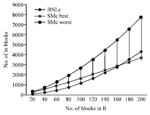 | |
| Fig. 2: | Block nested loop and sort-merge join |
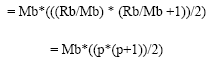
BNLc = Rb + Mb*(((Rb/Mb) * (Rb/Mb +1))/2) |
and so
Smcworst-case = ESc + BNLc |
The worst case occurs when we have one tuple at least in each sorted bock overlap with one or more tuples in the last block of the sorted relation.
The best case occurs when the SC = 1, in this case, for each outer loop we only read one block in InnerBuffer. So, the merging complexity will be:
Rb + (Rb/Mb) |
and so
Smcbest-case = ESc + (Rb + (Rb/Mb)*sc) Smcbest-case=(2*Rb)+(2*(Rb*(log2Rb)) + (Rb + (Rb/Mb)*sc) Smcbest-case= (3*Rb) + (Rb/Mb)*sc + (2*(Rb*(log2Rb)) |
Note that we have considered SC in our formulation for SMc, but we did not include SC in BNLc. This is because the tubles in BNL are not sorted.
Performance evaluation: Here, a graph showing the performance of the proposed algorithms will be presented. Fig. 2 shows the cost of the modified block nested loop join and Modified Sort-merge Join. We are using 2-way sort merge for external sorting and outerbuffer = 5.
From the cost formulas and the graph, three facts can be seen.
| • | Sort-merge join for overlap-join in the worst case is worse than the block nested loop overlap-join |
| • | Sort-merge join for overlap-join in the best case is better than the block nested loop overlap-join, but this is true when the relation r is big enough to overcome the sorting cost |
| • | SC and OC have big effect on the cost function in addition to the available buffer size |
CONCLUSION
Overlap-Join is an important operation in many applications and the cost of joining operations is very high in general. The standard algorithms cannot be used directly with acceptable performance for overlap-join. Modified nested block join and modified sort-merge join algorithms has been presented and cost function has been developed. Overlap coefficient and span coefficient has been developed and used in the cost functions. The study showed that using sort-merge is not more efficient than the nested block join especially when the span coefficient is high.
REFERENCES
- De Witt, D.J., J.F. Naughton and D.A. Schneider, 1991. An evaluation for non equi-join algorithms. Proceedings of the 17th International Conference on Very Large Data Bases, Sept. 3-6, San Francisco, CA, USA., pp: 443-452.
Direct Link - Gao, D., C.S. Jensen, R.T. Snodgrass and M.D. Soo, 2005. Join operations in temporal databases. VLDB J., 14: 2-29.
Direct Link - Saffarzadeh, M., I.N. Kamal Abadi, A.A. Kordani and E.A. Gangraj, 2008. A new approach in airport capacity enhancement based on integrated runway assignment and operations planning model. J. Applied Sci., 8: 4040-4050.
CrossRefDirect Link - Graefe, G., 1993. Query evaluation techniques for large databases. ACM Comput. Surveys, 25: 73-170.
Direct Link - Shen, H., 1995. An efficient permutation-based parallel algorithm for range-join in hypercubes. Parallel Comput., 21: 303-313.
Direct Link - Schikuta, E., 2003. Performance modeling of the grace hash join on cluster architectures. Proceedings of the 17th International Symposium on Parallel and Distributed Processing, April 22-26, Washington, DC, USA., pp: 276.2-276.2.
Direct Link - Sinha, M. and S.V. Chande, 2010. Query optimization using genetic algorithms. Res. J. Inf. Technol., 2: 139-144.
CrossRefDirect Link - Noh, S.Y. and S.K. Gadia, 2008. Benchmarking temporal database models with interval-based and temporal element-based timestamping. J. Syst. Software, 81: 1931-1943.
CrossRef - Soo, M.D., R.T. Snodgrass and C.S. Jensen, 1994. Efficient evaluation of the valid-time natural join. Proceedings of the 10th International Conference on Data Engineering, Feb. 14-18, Washington, DC, USA., pp: 282-292.
Direct Link