
Wang Xu
Southwest Electronics and Telecommunication Technology Research Institute, University of Electronic Science and Technology of China, Chengdu, China
He Zi-shu
Department of Electronic Engineering, University of Electronic Science and Technology of China, Chengdu, China
Information Technology Journal
Year: 2011 | Volume: 10 | Issue: 6 | Page No.: 1150-1160


ABSTRACT
According to the TOAs (time of arrival) of periodic signal of constant-speed moving target, this study proposes the algorithms to estimate its range, velocity, velocity components and position coordinates in the three-sensor TDOA (time different of arrival) location system. The traditional three-sensor TDOA positioning system can locate two-dimensional target but the result may be ambiguity or no solution. The unique solutions of velocity components and position coordinates of two-dimensional target can be obtained by using the method of Target Motion Analysis (TMA). For the target moving at a constant speed in three-dimensional space, we can make the two-valued estimations of its velocity components and position coordinates. Because the height value of a target flying in real space cannot be negative, we can position the target by excluding the false position. In simulation analysis, we have carried out contrastive analysis of the various algorithms and their estimation accuracies. The simulation results verify the validity of the proposed algorithms.
PDF Abstract XML References Citation
Received: February 01, 2011;
Accepted: March 19, 2011;
Published: May 13, 2011
How to cite this article
Wang Xu and He Zi-shu, 2011. Target Motion Analysis in Three-Sensor TDOA Location System. Information Technology Journal, 10: 1150-1160.
DOI: 10.3923/itj.2011.1150.1160
URL: https://scialert.net/abstract/?doi=itj.2011.1150.1160
DOI: 10.3923/itj.2011.1150.1160
URL: https://scialert.net/abstract/?doi=itj.2011.1150.1160
INTRODUCTION
In terms of multi-sensor TDOA (time different of arrival) positioning systems, the three-sensor TDOA positioning system is widely used because the system scale is accessible and its positioning accuracy can meet the demands of the trajectory estimation (Yong-Guang et al., 2004; Chao-Mou and Zhi-Qiang, 2009).
The three-sensor TDOA positioning algorithm (Foy, 1976; Chan and Ho, 1994; Huang and Lu, 2004) needs to solve nonlinear equations with the common methods of Taylor expansion method, two-step least square method, modified least square method, etc. Influenced by the factors of geometry disposition, noise and measurement errors of three stations, multiple solutions or no solution is common for three-station TDOA positioning algorithm (Chao-Mou and Zhi-Qiang, 2009). And such phenomenon is commonly eliminated by increasing stations and using the method of data fusion.
For single-sensor location algorithm, the Target Motion Analysis (TMA) is widely studied in the fields such as positioning algorithm (Zhong-Kang et al., 2008; Nardone and Graham, 1997; Moon and Nordone, 2000), observability of motion parameters (Nardone and Aidala, 1981; Fogel and Gavish, 1988; Song, 1996) and optimal maneuver strategy of observation station (Fawcett, 1988; Hammel et al., 1989) etc. The TMA aims to estimate the trajectory by using TOA of signal, bearing, Doppler shift and other types of measurements. In TMA, the characteristics of the constant-speed motion and the periodicity of signal are commonly used.
In the multi-sensor bearing-only target motion analysis, the target can be positioned by the combination of crossing location and target motion analysis. Iltis and Anderson (1996) and Tremois and Le Cadre (1996) have researched the methods of estimating the motion trajectory by using bearing-only measurements.
A target position algorithm is researched in this study by adopting the method of integrating three-sensor TDOA positioning and target motion analysis. Firstly, a model is established for target location and motion analysis in three-dimensional space. Secondly, the estimation algorithms of range and velocity are proposed according to the observability of TOA-only target motion analysis. Then, the observabilities of position coordinates and velocity components in two-dimensional and three-dimensional space are analyzed and the corresponding estimation algorithms are presented. Finally, the simulation analysis is made for the proposed algorithms.
ALGORITHM MODEL
Assuming that the positions of the three sensors are R1 (x01, y01, z01) R2 (x02, y02, z02) and R3 (x03, y03, z03), the target velocity is (vx, vy, vz).
 | |
| Fig. 1: | TMA for 3 sensors |
The three sensors receive the N+1 signals which are, respectively sent by the moving target on the positions of Tk, Tk-1, ... and Tk-N, as shown in Fig. 1. Suppose that the corresponding sending time of each signal is t t(k-j) (j = 0, 1,..., N) and the corresponding receiving time of the sensor i is tri (k-j) (i = 0, 1,..., N). The sending time interval of any two signals is a multiple of the signal cycle Ts.
The relationship between the receiving time and sending time is shown as:
| (1) |
where, c is the speed of light. The range from target at position Tk-j to the sensor i is rij:
| (2) |
For the first sensor, the receiving time difference between the signals of target at positions Tk-j and Tk-1 is:
| (3) |
where:
| (4) |
The r1j-r1l in (3) is the range difference between the target positions at Tk-j and Tk-l to the sensor 1 that is generally much smaller than the range of electromagnetic wave travelling in the signal cycle Ts. If the following condition is met:
| (5) |
Δm can be calculated by:
| (6) |
where, round () is rounding function.
According to (3), the range difference between the target positions at Tk-j and Tk-l to the sensor 1 is:
| (7) |
According to (4), the sending time difference between the signals of target positions at Tk-j and Tk-l is:
| (8) |
In the same way, the range difference between the target positions at Tk-j and Tk-l to the sensor 2 or 3 is:
| (9) |
| (10) |
According to Eq. 1, the range difference between the ranges from the target at position Tk-j to the sensor 1 and 2 is:
| (11) |
The range difference between the ranges from the target at position Tk-j to the sensor 1 and 3 is:
| (12) |
The Eq. 7, 9 and 10 are the models of the range difference of different signals to the same sensor, Eq. 11 and 12 are that of the range difference of the same signal to different sensors and Eq. 8 is that of the sending time difference of different signals.
OBSERVABILITY OF THE TARGET RANGE BASED ON MULTIPLE SENSORS
According to the model (11) of the range difference of the same signal to sensor 1 and 2 for the target position Tk-j, r2l is moved leftwards, dr1 is moved rightwards and then square it, the following formula is derived:
| (13) |
Using Eq. 2:
 | (14) |
In which the range from sensor to the coordinate origin is:
| (15) |
Let:
| (16) |
| (17) |
Eq. 14 is rewritten as:
| (18) |
To find the range of target at position Tk-j, by using (7), we can obtain:
| (19) |
The matrix equation is established by using N+1 measurements:
| (20) |
where:
 |
In the same way, according to the model Eq. 12 of the range difference of the same signal to sensor 1 and 3 for the target position Tk-l, if:
| (21) |
| (22) |
we can obtain:
| (23) |
where:
 |
The solvability conditions of Eq. 20 and 23 are:
| (24) |
and
| (25) |
When the target moves on the extension of the connecting line of two sensors, dr12j or dr13j is the distance between the two corresponding sensors and a constant for any j. In Eq. 20 or 23, the first and the third ranks of A1j or A2j are proportionate with a ratio coefficient of -dr12j or -dr13j, so neither Eq. 20 nor 23 has a solution.
The simultaneous Eq. 20 and 23 is:
| (26) |
where:
 |
The solvability condition of (26) is:
| (27) |
According to the characteristic of the constant-speed motion, the range r1j from the target to sensor 1 can be estimated from Eq. 20, 23 and 26 and then the ranges from the target to sensor 2 or 3 can be obtained from Eq. 11 and 12.
OBSERVABILITY OF THE TARGET RANGE AND VELOCITY BASED ON SINGLE SENSOR
In Eq. 7, r1l is moved leftwards, Δr1jl is moved rightwards and then square it, the following formula is derived:
| (28) |
Using Eq. 2, then:
| (29) |
Let:
| (30) |
| (31) |
| (32) |
where, v is the speed of target motion.
According to Eq. 8,
| (33) |
Eq. 29 is deformed as:
| (34) |
For any j, when; lε (0, 1, 2,..., N) and l ≠ j, N equations with the variable of r1j can be established.
In order to facilitate to express the matrix form in any j, it is also denoted with a equation in case of l = j, that is, there are N+1 equations to be established with the variable of r1j. The matrix form of equations is:
| (35) |
In which:
 |
For the sensor 2, let:
| (36) |
According to Eq. 9, then:
| (37) |
| (38) |
Where:
 |
For the sensor 3, let:
| (39) |
According to Eq. 10, then
| (40) |
| (41) |
Where:
 |
Eq. 35, 38 and 41 are the single-sensor range and velocity estimation algorithms to estimate target ranges and velocities based on the models of the range difference of different signals on the trajectory to the same sensor. When the corresponding ranks of matrix A4j, A5j and A6j are 3, the corresponding Eq. 35, 38 and 41 have solutions and we can estimate the range and velocity of target.
According to Eq. 11, use r1j to express r2j in Eq. 37, then:
| (42) |
According to Eq. 12, use r1j to express r3j in Eq. 40, then:
| (43) |
The simultaneous equation of 34, 42 and 43 is:
| (44) |
Where:
 |
Equation 44 uses the TOA measurements of three sensors to estimate the velocity and range from target to the first sensor. When the rank of matrix A7j is 5, Eq. 44 has a solution.
TMA OF TWO-DIMENSIONAL TARGET
For two-dimensional target, Eq. 16, 17, 21 and 22 are represented as:
| (45) |
| (46) |
| (47) |
| (48) |
The matrix equation of target position estimation is
| (49) |
Where:
The matrix equation of velocity components estimation is:
| (50) |
Where:
Matrix A8 in Eq. 49 is equal to A9 in Eq. 50. The solvability condition of (49) and (50) is:
| (51) |
Eq. 49 and 50 are solvable as long as three sensors are not at the same line in the two-dimensional space, i.e., the following condition is met:
| (52) |
Therefore, the target position coordinates and velocity components are observable making use of target motion analysis for two-dimensional target.
TMA OF THREE-DIMENSIONAL TARGET
Taking ordinate z as a known parameter, the (x, y) can be estimate using (16) and (21):
| (53) |
Where:
Supposed:
| (54) |
then:
| (55) |
Where:
| (56) |
The range r1j from target to the sensor 1 can be estimated according to the range observability. When j is equal to zero, from Eq. 2:
| (57) |
Substituting Eq. 55 into above equation, we can obtain:
| (58) |
Where:
 |
Solving Eq. 58, we can obtain two solutions of z:
| (59) |
Substituting Eq. 59 into Eq. 55, we can obtain two pairs of target position solutions (x1, y1, z1) and (x2, y2, z2) which one is real and the other is pseudo.
If the ordinates of the three sensors are the same:
| (60) |
The (x, y) can be get from (49)and then:
| (61) |
In view of the actual space region where the target appears, we take the solution with positive ordinate as the real one.
Taking vz as a known parameter, the (vx, vy) can be estimate using Eq. 17 and 22,
| (62) |
Where:
According to Eq. 54,
| (63) |
Where:
| (64) |
The v2 can be estimated according to the velocity observability. Substituting Eq.63 into 31, we can obtain:
| (65) |
Where:
 |
Solving Eq. 58, we can obtain two solutions of vz:
| (66) |
Substituting Eq. 66 into 63, we can obtain two pairs of solutions (vx1, vy1, vz1) and (vx2, vy2, vz2) which one is real and the other is pseudo.
If the ordinates of the three sensors are the same, the (vx, vy) can be get from Eq. 50 and then:
| (67) |
Once determining the true position (x, y, z), we can identify the true value of velocity components by using Eq. 30. The u5 can be estimated from velocity observability, we can use the search method shown in the following formula to determine the subscript i corresponding with the real velocity component:
| (68) |
SIMULATION OF TOA-ONLY TARGET MOTION ANALYSIS IN THREE-SENSOR SYSTEM
Assuming that three sensors are located at coordinates (0, 0, 0), (10000, 5000, 0) and (-10000, 5000, 0) and RMS error of sensor location coordinates is 3 m, that of range difference 30 m and that of target system synchronization 100 m (the range difference corresponding with the RMS error of signal cycle Ts). Suppose that a moving target sends a signal every 5 sec.
Simulation analysis of range estimation: Assuming that a target makes constant-altitude flight from left to right and parallel to the X-axis in three-dimensional space at the altitude of 8,000 m and the constant flight velocity of 200 ms-1 and the starting coordinate is (-100000, 50000, 8000). Figure 2 shows the ranges from the locations of the target trajectory to the three sensors.
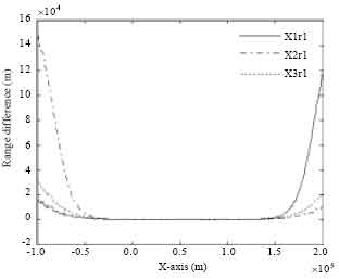
The estimation algorithms of r1, the range from the target to sensor 1, are as follows: dual-sensor TDOA algorithm X1r1 (Eq. 20) and X2r1 (Eq. 23), dual-sensor TDOA joint algorithm X3r1 (Eq. 26), single-sensor algorithm [X4r1 (Eq. 35] and single-sensor synchronization algorithm [X7r1 (Eq. 44)].
The simulation results in Fig. 3 and 4 are used to describe the biased characteristics of the estimation algorithms.
Figure 3 shows the differences between the real value r1 and the estimated values derived from the dual-sensor TDOA algorithms X1r1, X2r1 and X3r1. The results show that the algorithms of the dual-sensor TDOA algorithms X1r1, X2r1 and X3r1 are biased. The biased values increase with the increase of target range and the estimated values are smaller than the true ones. The biased value of algorithm X1r1 is smaller than that of algorithm X2r1 when the target moves from far to near, vice versa. The biased characteristic of algorithm X3r1 is between that of the algorithms X1r1 and X2r1.
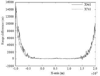
Figure 4 shows the differences between the real value r1 and the estimated values derived from single-sensor algorithms X4r1 and X7r1. The results show that the biased characteristic of single-sensor synchronization algorithm X7r1 is slightly better than that of single-sensor algorithm X4r1.
Comparing Fig. 3 with Fig. 4, we can conclude that the single-sensor algorithms have better biased characteristic than dual-sensor TDOA ones.
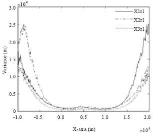
Figure 5 shows the estimated variances of dual-sensor TDOA algorithms X1r1, X2r1 and X3r1. The estimation accuracy of dual-sensor TDOA joint algorithm X3r1 is better than that of algorithms X1r1 and X2r1. The variance of algorithm X1r1 is smaller than that of algorithm X2r1 when the target moves from far to near, vice versa.
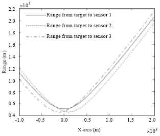 | |
| Fig. 2: | Ranges of the target to three sensors |
 | |
| Fig. 3: | Range differences between the real and estimated values of dual-sensor TDOA algorithms X1r1, X2r1 and X3r1 |
 | |
| Fig. 4: | Range differences between the real and estimated values of single-sensor algorithms X4r1 and X7r1 |
 | |
| Fig. 5: | Variances of dual-sensor TDOA algorithms X1r1, X2r1 and X3r1 |
 | |
| Fig. 6: | Variances of dual-sensor TDOA algorithm X3r1, single-sensor algorithms X4r1 and X7r1 |
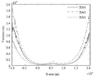
Figure 6 shows the estimated variances of dual-sensor TDOA algorithm X3r1, single-sensor algorithms X4r1 and X7r1. For the single-sensor algorithms X4r1 and X7r1, the estimation accuracy of algorithm X7r1 is better than that of algorithm X4r1. For the single-sensor synchronization algorithm X7r1 and dual-sensor TDOA joint algorithm X3r1, the estimation accuracy of algorithm X7r1 is also better than that of algorithm X3r1.
Simulation analysis of velocity estimation: The following velocity estimation algorithms are discussed in this paper: sensor 1 algorithm X4v (Eq. 35), sensor 2 algorithm X5v (Eq. 38), sensor 3 algorithm X6v (Eq. 41) and single-sensor synchronization algorithm X7v (Eq. 44).
Figure 7 shows the velocity estimation accuracy analysis of algorithms X4v, X5v, X6v and X7v. For the single-sensor algorithms X4r1, X5r1 and X6r1, every algorithm have better accuracy situation than others during the target motion.
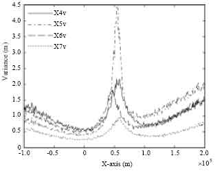 | |
| Fig. 7: | Velocity variances of algorithms X4v, X5v, X6v and X7v |
 | |
| Fig. 8: | Estimation variances of variable u1 |
The estimation accuracy of single-sensor synchronization algorithm X7v is better than that of other single-sensor algorithms X4v, X5v and X6v.
We can also generalize a conclusion from Fig. 7 that the velocity estimation accuracies of all the four algorithms will be local maximum values when the target trajectories are nearness to the shortest range to the three sensors.
Simulation analysis of two-dimensional target location estimation: The position estimation accuracy is expressed by GDOP (Geometric Dilution of Precision):
| (69) |
In which σ2x, σ2y are estimated RMS values of coordinates x and y.
Assuming that a two-dimensional target makes flight from left to right and parallel to the X-axis at the constant velocity of 200 m s-1 and the starting coordinate is (-50000, 50000).
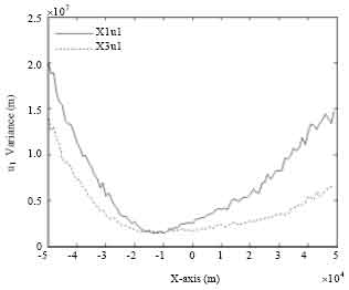
For the two-dimensional target location algorithm of Eq. 49, the intermediate variables u1 and u3 are needed. The estimation algorithms of u1 are dual-sensor TDOA algorithm X1u1 (Eq. 20) and dual-sensor TDOA joint algorithm X3u1 (Eq. 26). As shown in Fig. 8, the algorithm X3u1 has the better estimation accuracy than X1u1. Therefore, the estimated value derived from algorithm X3u1 is used to position the target.
The estimation accuracy of intermediate variable u3 is shown in Fig. 9. The algorithm X3u3 is chose to position the target.
Figure 10 shows the contrastive analysis of the estimated and true trajectory with a basic agreement. Thus, the target location algorithm of Eq. 49 can position two-dimensional target.
Figure 11 shows the location estimation accuracy. We can get a conclusion that the smaller the range is, the better the estimation accuracy will be.
Simulation analysis of three-dimensional target location estimation: The three-dimensional position estimation accuracy is estimated by GDOP:
| (70) |
In which σ2x, σ2y and σ2z are estimated RMS values of coordinates x, y and z.
Besides the intermediate variables u1 and u3, the range u10 is required for locating three-dimensional target using location algorithms of Eq. 55 and 59. According to the results of above range simulation analysis, the algorithm X7r1 is used to position the three-dimensional target.
Figure 12 and 13 show the simulation results of a target motion parallel to the horizontal axis with y-axis 50 km and Z-axis 8000 m. Figure 12 shows the contrastive analysis of the estimated and true trajectory of target. Figure 13 shows the contrastive analysis of location estimation accuracy and the estimation accuracy of range r10 derived from algorithm X7r1.
Figure 12 shows a basic agreement between the estimated and real trajectory. Therefore, the target location algorithms of Eq. 55 and 59 can position three-dimensional target.
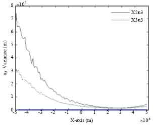 | |
| Fig. 9: | Estimation variances of variable u3 |
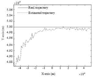 | |
| Fig. 10: | Target real and estimated trajectories |
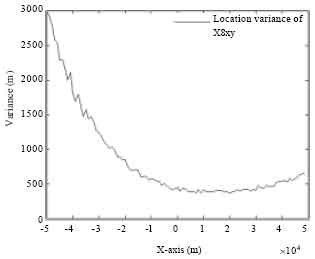 | |
| Fig. 11: | Variance of target location |
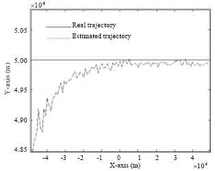 | |
| Fig. 12: | Target real and estimated trajectories in X-Y plane |
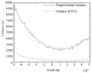 | |
| Fig. 13: | Variance of target location |
As shown in Fig. 13, the smaller the range is, the better the estimation accuracy will be and the variance of algorithm X7r1 is smaller than that of target location.
CONCLUSION
This study, based on the characteristics of target motion and the TOAs of the periodic signal, researches the position algorithm for the two- and three-dimensional target in three-station location system. The main conclusions are as follows:
| • | The unique solutions of position coordinates and velocity components of two-dimensional target can be found by solving linear equations and the shortcomings of multiple solutions or no solution of the traditional TDOA positioning algorithm can be avoided |
| • | For three-dimensional target, the algorithms proposed in this paper can make two-valued estimations of velocity components and position coordinates, and we can obtain two trajectories which one is false. The height value of false trajectory is negative while a certain condition is met, for instance, the heights of the three stations are the same value; the true trajectory can be uniquely identified based on the space region where the target may occur |
REFERENCES
- Chan, Y. and K.C. Ho, 1994. A simple and efficient estimator for hyperbolic location. IEEE Trans. Signal Process., 42: 1905-1915.
CrossRef - Yong-Guang, C., L. Chang-Jin and L. Xiu-He, 2004. A precision analyzing and reckoning model in tri-station TDOA location. Acta Electronica Sinica, 32: 1452-1455.
Direct Link - Fawcett, J.A., 1988. Effect of course maneuvers on bearings-only range estimation. IEEE Trans. Acoustics Speech Signal Process., 36: 1193-1199.
CrossRef - Fogel, E. and M. Gavish, 1988. Nth-order dynamics target observability from angle measurements. IEEE Trans. Aerospace Electron. Syst., 24: 305-308.
CrossRef - Foy, W.H., 1976. Position-location solutions by Taylor series estimation. IEEE Trans. Aerospace Electron. Syst., 12: 187-194.
CrossRef - Hammel, S.E., P.T. Liu, E.J. Hilliard and K.F. Gong, 1989. Optimal observer motion for localization with bearings measurements. Comput. Math. Appl., 18: 171-180.
CrossRef - Huang, Z. and J. Lu, 2004. Total least squares and equilibration algorithm for range difference location. Electron. Lett., 40: 323-325.
CrossRef - Nardone, S.C. and V.J. Aidala, 1981. Observability criteria for bearings-only target motion analysis. IEEE Trans. Aerospace Electron. Syst., 17: 162-166.
CrossRef - Nardone, S.C. and M.L. Graham, 1997. A closed-form solution to bearing-only target motion analysis. IEEE J. Oceanic Eng., 22: 168-178.
CrossRef - Tremois, O. and J.P. Le Cadre, 1996. Target motion analysis with multiple arrays: Performance analysis. IEEE Trans. Aerospace Electron. Syst., 32: 1030-1046.
CrossRef - Iltis, R.A. and K.L. Anderson, 1996. A consistent estimation criterion for multisensor bearings-only tracking. IEEE Trans. Aerospace Electron. Syst., 32: 108-120.
CrossRef - Song, T.L., 1996. Observability of target tracking with bearings-only measurements. IEEE Trans. Aerospace Electron. Syst., 32: 1468-1472.
CrossRef