
O.I. Shittu
Department of Statistics, University of Ibadan, Ibadan, Nigeria
D.K. Shangodoyin
Department of Statistics, University of Ibadan, Ibadan, Nigeria
Asian Journal of Scientific Research
Year: 2008 | Volume: 1 | Issue: 2 | Page No.: 130-137


ABSTRACT
We consider the identification and detection of outliers in frequency domain using the spectral method. By assuming both the additive and multiplicative effect of outliers on a series, the parameters of the model were estimated using the maximum likelihood method with a view to measuring the effect of the suspected outlier on the parameter of the series. The occurrence of outliers has led to a shift in the phase and amplitude of the Fourier series thus affected the periodogram estimates. Further more, detection of aberrant observations is more exact in the frequency domain than in the time domain.
PDF Abstract XML References Citation
How to cite this article
O.I. Shittu and D.K. Shangodoyin, 2008. Detection of Outliers in Time Series Data: A Frequency Domain Approach. Asian Journal of Scientific Research, 1: 130-137.
DOI: 10.3923/ajsr.2008.130.137
URL: https://scialert.net/abstract/?doi=ajsr.2008.130.137
DOI: 10.3923/ajsr.2008.130.137
URL: https://scialert.net/abstract/?doi=ajsr.2008.130.137
INTRODUCTION
Considerable attention has been devoted to the detection of outliers in discrete univariate time series were developed for univariate samples in time domain. Fox (1972) and Rosner (1975) started study on outlier detection, Haoglin and Iglewicz (1987) worked on resistant rules for labeling outliers. Chang and Tiao (1983) introduced the additive (AO) and Innovative (IO) models, these were further developed by Shangodoyin and Shittu (2000) the Multiplicative (MO) and Convolution (CO) were proposed in using the model identification tools (ACF and PACF). However in almost all the techniques in time domain Tsay (1986). Shangodoyin and Shittu (2003) detected that outliers were found to have some degree of smearing or swamping effects on other regular observations in the series. Also most economic and social data which are no longer linear but continuous in nature just in physics, engineering and medicine are of the continuous type which can be analyzed in frequency domain.
In this research, we determine the occurrence of outliers in time series data that assumes a Gaussian process and has a continuous spectrum using the spectral method of analysis. An algorithm that uses the robust trigonometric regression of Tatum and Hurvich (1993) is proposed. The estimate of the parameters of the model for the contaminated series is obtained by the maximum likelihood method with a view to compare with that obtained by the least squares method by Priestley (1981)and Brillinger (1981). We also assume the additive and multiplicative effect of outliers on the observed process and the measure of impact of outliers on the observed process and the measure of impact of outliers on the observed values shall be estimated as well as the location of the suspected outlier using a proposed algorithm based on the repeated median transform of Siegel (1982).
ESTIMATION OF PARAMETER USING THE MAXIMUM LIKELIHOOD TECHNIQUE
Here, we estimate the parameters of the model using the maximum likelihood technique with a view to comparing them with that obtained by the least Square method in the literature (Priestley, 1981; Brillinger, 1981).
Let Xt be any periodic stochastic process with period 2π with Fourier representation as:
| (1) |
Where:
| wi: | The Fourier frequency; |
| φi: | The phase uniformly distributed on (0, 2π) |
| Ri: | The amplitude |
| εt: | The random error term NID (0, σ) |
Equation 1 can be re-written as:
| (2) |
Ai = Rj cos φi and Bi = Rj sin φi are parameters to be estimated and εt is a purely random process, normal and independently distributed with:
Where, σε2 is a further unknown parameter and
Since εt ~ N I D (0, σ2) the distribution function of εt can be given as:
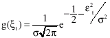 | (3) |
With a corresponding maximum likelihood function:
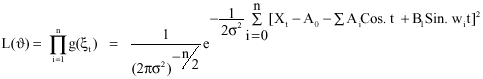 |
and log- likelihood:
| (4) |
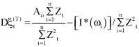
The maximum likelihood estimate of the Ao, Ai and Bi are
| (5) |
| (6) |
and
| (7) |
It can be shown that the estimates ![]() are unbiased with variances:
are unbiased with variances:
and
Where:
is the unbiased estimate of the residual variance.
ESTIMATION OF PARAMETERS OF A CONTAMINATED SERIES
Our focus here is to derive estimates of the parameters of outlier contaminated series.
The Additive Model
Suppose outliers have additive effect on a series, we assume the additive outlier generating model of Tsay (1986).
The additive model is given by:
| (8) |
Where, Xt is the observed series; Zt is the outlier free series; and D is the magnitude of the outlier ![]() is the time indicator of the outlier such that
is the time indicator of the outlier such that
Using (8) in (4) gives the maximum likelihood function:
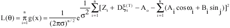 | (9) |
and the log-likelihood function:
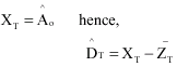
The maximum likelihood estimate of the Ao is:
| (10) |
the estimate of the magnitude of outlier is:
| (11) |
at ![]() therefore:
therefore:
| (12) |
and for reasons of orthogonality when there is no outlier:
 | (13) |
The maximum likelihood estimate of the Ai and Bi are:
| (14) |
and
| (15) |
It could be observed that from (12), (14) and (15) the occurrence of outlier has influenced only ![]() (the grand mean) and no influence on
(the grand mean) and no influence on ![]() for (AO) model. However, the influence on
for (AO) model. However, the influence on ![]() could be monotone increasing or decreasing depending on whether
could be monotone increasing or decreasing depending on whether ![]() is positive or negative.
is positive or negative.
Thus the occurrence of outlier in any series does not affect the periodogram ![]() for the (AO) model.
for the (AO) model.
The Multiplicative Model (MO)
Suppose outlier have multiplicative effect on a data set, without loss of generality, we consider the multiplicative outlier generating model (MO) (Shangodoyin and Shittu, 2003):
| (16) |
Where, Xt is the observed series; Zt is the outlier free series; and D is the magnitude of the outlier ![]() is the time indicator of the outlier such that
is the time indicator of the outlier such that
Using (16) in (4) we have the log-likelihood function:
| (17) |
and the estimate of:
| (18) |
| (19) |
While the MLE of the magnitude of outlier for the multiplicative model is:
 | (20) |
Where:
the Normalized Periodogram.
The maximum likelihood estimate of the Ai and Bi are:
| (21) |
and
| (22) |
However when there is no outlier, that is when t # T and ![]() = 0, the estimates of
= 0, the estimates of ![]() are
are
and
respectively.
Which are also unbiased
DETECTION OF OUTLIERS USING THE DERIVED ESTIMATES
The derived estimates shall now be used to diagnose for suspected outliers using the following proposed algorithms.
Algorithm I (Detection of Outlier)
If observations X1, X2,. . . . ; XN can be expresses as a sum of sine and cosine waves as in (2) which can be written as:
Using any of the spread sheet package or Microsoft Excel to
| • | Obtain the estimate of the Fourier frequencies |
| • | i = 1, 2, . . . k hence the periodogram IN(ωi) for all ω in the range |
Where, α(ω) and β(ω) are as defined in (9) and (10).
If ![]() is very close to its true value then
is very close to its true value then ![]() and
and ![]() will also be close to
will also be close to ![]() respectively, hence the squared amplitude will be non-zero. However, if
respectively, hence the squared amplitude will be non-zero. However, if ![]() is substantially far from its expected value the periodogram will be close to zero.
is substantially far from its expected value the periodogram will be close to zero.
| • | Determine the value of ωi; i = 1, 2,. . . . K whose squared amplitude is non-zero. |
| Obtain the residual variance and Compute the test statistics: |
| • | Determine λF = Max(1<F<N) λi |
| • | For all λFi > C where, C is the critical value simulated as 1.00 or 1.10, the observation Xts corresponding to λFi is declared an outlier for the Fourier frequencies ωi; i = 1, 2,.... k whose squared amplitude is non-zero. |
| • | Use the Repeated median filter of Siegel (1982) and for all ωi ≠ 0; compute the estimate discrete Fourier transform: |
| * | XtF gives the uncontaminated data set whose contamination/outlier has been removed. |
DATA ANALYSIS
To show the use of the above algorithm, five different natural and well analysed data were used. They are series A: Zadakat data in a local mosque in Nigeria; series B: Wolfer Sunspot data, a record of activities in the solar system; series C: Batch chemical data; series D: Well analyzed data from Box and Jenkins (1976). Nigerian Consumer Price index data obtained for the Federal Office of Statistics; and series E: Diabetic patient data from the University teaching Hospital, Ibadan, Nigeria.
The algorithm I was used to diagnosed collected data for outliers using the Microsoft Excel package and the results were summarized in the Table 1-3.
| Table 1: | The timing and magnitude of outliers |
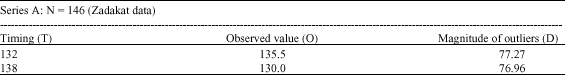 | |
| Table 2: | The timing and magnitude of outliers |
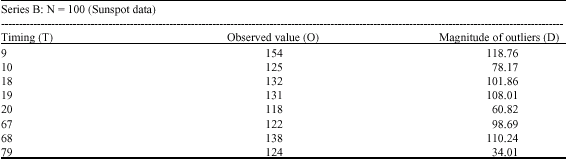 | |
| Table 3: | The timing and magnitude of outliers |
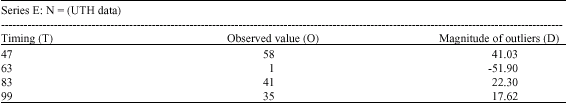 | |
| It should be noted that no outlier were detected in series C (N = 48) and series D (N = 70) | |
CONCLUSIONS
The derived estimates using the Maximum Likelihood Method (MLE) compares favourably with the Least Squares Method (LSM). This confirms the remark made by Priestley (1981) that Maximum likelihood method is a more asymptotically fully efficient method of estimation. It was found out that the contamination has no influence on the estimates of ![]() and
and ![]() for (AO) model. However, the influence on
for (AO) model. However, the influence on ![]() could be monotone increasing or decreasing depending on whether
could be monotone increasing or decreasing depending on whether ![]() is positive or negative, however for the multiplicative model, the influence on the parameter estimates were noticeable under the null hypothesis that there is contamination in the series.
is positive or negative, however for the multiplicative model, the influence on the parameter estimates were noticeable under the null hypothesis that there is contamination in the series.
We found that 2, 6 and 4 observations were identified as outliers in series A, B and E, respectively as shown in Table 1-3 while no observation were identified in series C and D. This is not to say that the algorithm can not work for small sample size data (i.e., n<100) as studies have shown that the procedure performs efficiently in any series were contamination is apparent.
It was also observed that using the spectral method of analysis in the frequency domain, the detection of aberrant observations were more exact than in those techniques in discrete domain.
With the Robust repeated median transform, it can also be observed that the issue of swamping or masking effect does not arise as outlying observations can be detected more exactly. The Robust repeated median transform technique is more complex and involves a lot of iterations; it is also more extensive computationally than other techniques.
RECOMMENDATIONS
Because of the fact that the number of outliers present in a set of data can not be determined aprori, it is recommended that every set of data, especially time series data should be diagnosed for outliers; the detected outlier should be treated or accommodated by any known method, before further analysis could be carried out.
Future research should emphasize on the identification and detection of outliers in Multivariate and categorical data as well as the extension of multiple outlier detection technique to the frequency domain.
REFERENCES
- Hoaglin, D.C. and B. Iglewicz, 1987. Fine-tuning some resistant rules for outlier labeling. J. Am. Stat. Assoc., 82: 1147-1149.
CrossRefDirect Link - Priestley, M.B., 1981. Spectral Analysis and Time Series. 1st Edn., Academic Press, London, ISBN-10: 0125649010, pp: 653.
Direct Link - Tatum, L.G. and C.M. Hurvich, 1993. High breakdown methods of time series analysis. J. R. Stat. Soc., 55: 881-896.
Direct Link - Tsay, R.S., 1986. Time series model specification in the presence of outliers. J. Am. Stat. Assoc., 81: 132-141.
CrossRefDirect Link