
Binod Kumar Singh
University of Petroleum and Energy Studies, Dehradun, India
LiveDNA: 91.4210
ORCID: 0000-0002-2215-8568
Asian Journal of Mathematics & Statistics
Year: 2015 | Volume: 8 | Issue: 1 | Page No.: 35-45


ABSTRACT
The loss function or cost function is a principal component of all optimizing problems such as statistical theory, decision theory, policy making, estimation process, forecasting, learning, classification and financial investment. In this study various types of loss functions and their uses were studied. In this study linex loss function, the analyst’s loss function, the optimal prediction under asymmetric loss, loss functions for forecasting financial returns, loss function and forecast biasedness, loss functions for estimation and evaluation, loss functions for probability forecasts and volatility forecasts have been studied. Further loss function for testing Granger-causality and loss function for uncertainty and policy aggressiveness have been also studied. This study suggested that among asymmetric loss functions linex loss function is more useful and to be applied in many financial situations.
PDF Abstract XML References Citation
Received: February 11, 2016;
Accepted: March 18, 2016;
Published: May 14, 2016
How to cite this article
Binod Kumar Singh, 2015. Loss Functions in Financial Sector: An Overview. Asian Journal of Mathematics & Statistics, 8: 35-45.
DOI: 10.3923/ajms.2015.35.45
URL: https://scialert.net/abstract/?doi=ajms.2015.35.45
DOI: 10.3923/ajms.2015.35.45
URL: https://scialert.net/abstract/?doi=ajms.2015.35.45
INTRODUCTION
A loss function usually called cost function is used in various optimization techniques in the area of statistical theory1, decision theory and machine learning is a function that plots an event or values of one or more variables in a real number and representing some cost associated with the event. An optimization problem always seeks to minimize a loss function. An objective function is either a loss function or its negative (sometimes called a reward function or a profit function or a utility function, etc.) and in all cases loss functions is to be maximized.
A main problem in statistical theory is to find necessary and sufficient condition for the consistency of an empirical risk minimization problem. Traditionally, the role played by the loss function is marginal and the choice of which loss to use for which problem is usually regarded as a computational issue (Vapnik, 1995, 1998; Alon et al., 1993; Cristianini and Taylor, 2000).
Most statistical theories are defined in terms of loss functions in the understanding that loss functions defined what a "Good" estimator or a "Good" predictor. The choice of a loss function cannot be formalized as a solution of a mathematical decision problem. Such type of decision problem would require the specification of another loss function. Therefore, the choice of a loss function requires familiar decisions, which necessarily have to be particular or at least contain particular elements.
The present study is focused on use of loss functions in the financial sector. To meet this objective different types of loss function under different conditions were discussed. This study suggested that linex loss function is a most appropriate function among loss functions used in different financial applications.
LOSS FUNCTION
Let us assume a set A is the set of all likely movements and a decision rule as a function δ: X→A. A loss function is a real lower-bounded function L on Θ×A for some θεΘ (Nikulin, 2001). The value L (θ, δ (X)) is the cost of action δ (X) under parameter θ. The value of the loss function is a random variable, since it depends on the outcome of a random variable X. The expected loss is obtained by taking the expected value with respect to the probability distribution Pθ of the observed data X. This is also referred to as the risk function of the decision rule δ and the parameter θ (Nikulin, 2001; Berger, 1985; DeGroot, 2004). The decision rule depends on the outcome of X. Thus the risk function is given by:
R (θ, δ) = EθL (θ, δ (X)) = ∫x L (θ, δ (X))dPθ (x)
Where:| θ | = | Fixed but possibly unknown state of nature |
| X | = | Vector of observations stochastically drawn from a population |
| Eθ | = | Overall expectation population values of X |
| dPθ | = | Probability measure over the event space of X, parametrized by θ and the integral is evaluated over the entire support of X |
But, in Bayesian approach, the expectation is calculated using the posterior distribution2 π* of the parameter θ:
![]()
For a scalar parameter θ, a decision function whose output ![]() is an estimate of θ and a quadratic loss function is L (θ,
is an estimate of θ and a quadratic loss function is L (θ, ![]() ) = (θ-
) = (θ- ![]() )2 and then the risk function becomes the Mean Square Error (MSE) of the estimate i.e., R (θ,
)2 and then the risk function becomes the Mean Square Error (MSE) of the estimate i.e., R (θ, ![]() ) = Eθ (θ-
) = Eθ (θ- ![]() )2.
)2.
In case of density estimation3, the unknown parameter is a probability density function. The loss function is typically chosen to be a norm in an appropriate function space. For example, for L2 norm4:
![]()
The risk function becomes the mean integrated square error, i.e., R (f, ![]() ) = E | | f-
) = E | | f- ![]() | |2.
| |2.
USES OF LOSS FUNCTION
| • | Loss function is used in predicting problems and depending on predicted and the observed value that defines the quality of a prediction |
| • | Loss function is used in estimation problems and depending on the true parameter and the estimated value it defines the quality of estimation. The true parameter value in an estimation problem is generally unobservable, while in a prediction problem the "Truth" is observable in the future |
| • | Many estimators such as method of least squares or M-estimators (broad class of estimators, which are obtained as the minima of sums of functions of the data) are defined as optimizers of certain loss functions which depends on the data and the estimated value |
| • | Loss function is used in defining optimal testing procedures |
| • | Loss function is used in Bayesian risk |
Besides general loss functions, the square loss function is used in a vast majority of applications of prediction and estimation problems (UMVU estimation is a restricted optimization of a square error loss function). Bayesian analysis is combined with decision analysis via explicit recognition of a loss function.
LINEX LOSS FUNCTION-A TYPE OF ASYMMETRIC LOSS FUNCTION
The symmetric quadratic function is the major loss functions for the evaluation of forecast. The loss remains same under negative and positive forecast errors. In such situation symmetric quadratic function is appropriate since mathematically it is very docile but from an economic point of view, it is not so straightforward. For a given set of data and under a quadratic loss, the optimal forecast is the conditional mean of the variable under study. In case of optimal forecast construction there is necessary to choose an appropriate loss function. Granger (1999) stated that for an asymmetric loss function, the optimal forecast would be more complex as it will depend not only on the choice of the loss function but also on the features of the probability density function of the forecast error. Granger (1999) transcripted the desirable majority of forecast work and used the cost function c (e) = ae2, a>0, largely for mathematical convenience. The loss function is a decisive constituent in all optimizing problems, such as statistical theory, decision theory, policy making, estimation, forecasting, learning, classification and financial investment, etc. In all such cases an asymmetric loss function is often relevant.
In the context of real estate assessment Varian (1975) proposed an asymmetric loss function called linex loss function (linear-exponential) as Eq. 1:
| (1) |
where, a, c>0 and ![]() . Also, here μ is the population mean and
. Also, here μ is the population mean and ![]() is the estimate of μ.
is the estimate of μ.
Zellner (1986) pointed out that if c = a then the Eq. 1 is minimized at Δ = 0. With this restriction Eq. 1 reduces to Eq. 2:
| (2) |
Zellner (1986) pointed out that for negative values of a linex loss retains its linear-exponential character and for small values of | a | linex loss is nearly symmetric and approximately proportional to square error loss. But for larger value of | a | it is quite asymmetric.
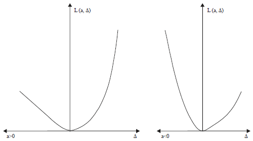 | |
| Fig. 1: | Linex loss function |
The other form of linex loss function (Fig. 1) is given in Eq. 3:
 | (3) |
where, a and b are shape and scale parameter respectively. If | a |→0, linex loss reduces to square error loss:
L (a, Δ) = b (eaΔ-aΔ-1)
Linex loss function is used in the field of hydrology in the estimation of peak water level in the construction of the dam. Linex loss function can be used with an appropriate value of ‘a’ (<0) in the construction of a dam where underestimation of the height of the dam is more serious than overestimation. In the above case, overestimation represents a conservative error which increases construction costs, while underestimation corresponds to the much more serious error in which overflows might lead to huge damage in the adjacent area. In case of dam construction an underestimate of the peak water is usually much more serious than an overestimate (Zellner, 1986).
Linex loss function can be used with an appropriate value of ‘a’ in the area of marketing strategy by using the exponential survival model, where ‘X’ is the lifetime of a component with a probability density function f (x; μ, σ) = (1/σ) exp {-(x-μ)/σ}, where μ is minimum guarantee/warranty time/period and 1/σ is failure rate.
Linex loss function can also be used with an appropriate value of ‘a’ (>0) for testing the reliability of equipments. The exponential life time of equipments, where X is the life of an equipment with a probability density function f (x; θ) = (1/θ) exp {-x/θ} such that the reliability function R (t) is given by: R (t) = P [X>t] = ![]() where, the overestimation of the reliability function can have marked consequence than under estimation.
where, the overestimation of the reliability function can have marked consequence than under estimation.
Linex loss function can also be used in following situations:
| • | The cost of arriving 10 min early in the airport is quite different from arriving 10 min late |
| • | The loss of booking a lecture room that is 10 seats too big for your class is different from that of a room that is 10 seats too small |
ANALYST’S LOSS FUNCTION
The financial analyst’s usually forecast corporate incomes, which is an important part and also contribute to investor’s decision models. There is a sufficient indication which suggests that the analyst’s forecasts are unscientific specifically when they appear to be biased (ex-post forecast errors have a non-zero mean) and inefficient (ex-post forecast errors are correlated with information known at the forecast date). Kothari (2001) has proposed two elucidations for such findings, both of which is based on the idea that the statistical bias and inefficiency of forecast is rational and originates in the loss functions sustaining analyst’s forecast decisions, i.e., how analysts weight prospective prediction errors when deciding on "Optimal" forecasts. Gu and Wu (2003) and Basu and Markov (2004) suggested that analysts have symmetric and linear loss functions. The analysts have an asymmetric loss functions, perhaps motivated by private incentives originating in business relationships between securities firms and their investment banking clients or in analyst’s dependence on managers for information (Lin and McNichols, 1998; Dugar and Nathan, 1995; Lim, 2001; Hong and Kubik, 2003). Research report of Friesen and Weller (2012) and McNichols and O’Brien (1997) is also consistent with both explanations but does not test the linear loss explanation against the asymmetric loss alternative. Clatworthy et al. (2012) also suggested that analyst’s earnings forecasts are driven by asymmetric loss functions, rather than by linear loss function.
From an investor point of view, it is better to understand the nature of the analyst’s loss function. An persuasive earnings forecast depends on both the analyst’s individual probability distributions of earnings and on the analyst’s loss function. Although, it is an investor’s loss function that ultimately determine investment decisions, interpretation and use of analyst’s forecasts by investors should reflect beliefs concerning analyst’s loss functions (Lambert, 2004). A rational analyst with a quadratic loss function minimizes the mean square value of predicted forecast errors (Mean square error) and in such situation the optimal forecast is the conditional mean of earnings and the expected value of the mean forecast error is zero, while the median forecast error depends on the distribution of earnings. Similar to a quadratic loss function, a symmetric linear loss function is symmetric in weighted positive and negative forecast errors of the same magnitude but it attaches less weight to extreme forecast errors. According to Granger (1969) in contrast to the quadratic loss function case, a rational analyst with a symmetric linear loss function minimizes the mean absolute value of anticipated forecast errors (Mean absolute error), the optimal forecast is the conditional median and the expected value of the median forecast error is zero, while the mean forecast error depends on the distribution of earnings. Granger (1969) proposed a linear-linear (LIN-LIN) loss function that weights positive and negative forecast errors of similar magnitude differently. But in the case of asymmetric loss functions, optimal forecasts are consistent with neither the Mean Square Error (MSE) nor Mean Absolute Error (MAE) criteria and both mean and median forecast errors can have expected values different from zero (Keane and Runkle, 1998).
The analysts produce forecasts consistent with asymmetric loss functions against the alternative of the symmetric loss (either quadratic or linear) and it is based on theoretical predictions relating forecast errors to the variance and skewness of the forecast error distribution. Gu and Wu (2003) inferenced that the magnitude of forecast errors depends on the skew ness of the earnings distribution because analysts have symmetric-linear loss functions. Consistent with this prediction, Gu and Wu (2003) explained that forecast errors are positively associated with earnings skew ness. The loss functions belong to the linex class of asymmetric loss functions introduced by Varian (1975) and Zellner (1986). Varian (1975) used linex loss function when there is a natural imbalance in the economic results of estimation errors of the same magnitude. It is a rational manner to formulate the consequences of estimation errors in real estate assessment. Underassessment results in an approximately linear loss of revenue, whereas overassessment often results in appeals with an attendant, substantial litigation and other cost. Under linex loss function where forecast errors are usually predicted to depend on the variance of the forecast error and when the distribution of forecast errors is conditionally non-normal, then forecast errors under linex loss function also depend on higher moments, including skew ness. The linear (MAE) loss function is a special limiting case in which forecast errors depend only on skew ness. Therefore, it’s dependence on forecast errors on the forecast error variance under asymmetric loss functions but not under linear loss functions. Clatworthy et al. (2012) stated that the forecast error variance dominates over forecast error, skew ness and this is also consistent with financial analysts, minimizing asymmetric loss functions. Forecast bias is also associated with book-to-price and market capitalization and again Clatworthy et al. (2012) suggested that the dominant role of forecast error variance in explaining the forecast bias is robust across characteristic portfolios.
OPTIMAL PREDICTION UNDER ASYMMETRIC LOSS FUNCTION
Christoffersen and Diebold (1996, 1997) used linex loss function in a study of optimal point prediction where different asymmetric loss functions are tested. A moment’s reflection yields the insight that prediction problems involving asymmetric loss structures arise routinely as a innumerable of situation-specific factors may reduce positive errors more (or less) costly than negative errors. Granger and Newbold (1986) noted that although an assumption of symmetry about the conditional mean is likely to be an easy one to accept,… an assumption of symmetry for the cost function is much less acceptable.
Granger (1969) studied Gaussian processes and shows that under asymmetric loss the optimal predictor is the conditional mean plus a constant bias term. Granger’s fundamental result, however, has two key limitations. First, the Gaussian assumption implies a constant conditional prediction-error variance. This is unfortunate because conditional heteroscedasticity is widespread in economic and financial data. Second, the loss function must be of the prediction error form.
LOSS FUNCTIONS FOR FORECASTING FINANCIAL RETURNS
Hong and Lee (2003) has used loss function in evaluating the point forecasts of financial returns and established mathematical function for square error loss, absolute error loss and trading return. The out-of-sample mean of these loss functions are the Mean Square Forecast Errors (MSFE), Mean Absolute Forecast Errors (MAFE) and Mean Forecast Trading Returns (MFTR). These loss functions also further include issues such as interest differentials, transaction costs and market depth since the investors are ultimately trying to maximize profits rather than minimize forecast errors, MSFE may not be the most appropriate evaluation criteria. Granger (1999) emphasized the importance of model evaluation using economic measures such as MFTR rather than statistical criteria such as MSFE and MAFE.
LOSS FUNCTION AND FORECAST BIASEDNESS
There are two rudiments of the forecasting process which determine whether the rational or an optimal earnings forecast is biased: The analyst’s loss function and the subjective probability distribution of earnings. If the subjective probability distribution of earnings is skewed, rational forecasts produced by analysts with symmetric loss functions are biased, unless the loss function is quadratic (Gu and Wu, 2003; Basu and Markov, 2004). However, earnings skew ness is not necessary for optimal forecasts to be biased because of the role played by the analyst’s loss function. While, Christoffersen and Diebold (1997) showed that closed form solutions for an optimal forecast cannot be developed for general asymmetric loss functions, the properties of optimal forecasts have been analyzed for two specific asymmetric loss functions viz., linear-linear (LIN-LIN) and linex (Granger, 1969).
Granger (1969) demonstrated that even if the data generating process for a variable follows an unconditional Gaussian process, optimal forecasts will exhibit constant bias when the forecaster optimizes with reference to an asymmetric, linear-linear (LIN-LIN) loss function. In such case the constant marginal loss (or cost) associated with a unit forecast error above some brink (e.g., zero) is different from the constant marginal loss for a unit forecast error below the same threshold. The magnitude of the optimal bias depends on the parameters of the loss function and on the forecast error variance. Christoffersen and Diebold (1996, 1997) extended Granger’s analysis of conditional Gaussian processes. In this case, optimal forecasts exhibit time-varying bias, conditional on the time-varying forecast error variance.
LOSS FUNCTION FOR ESTIMATION AND EVALUATION
Sometimes forecasting is based on an econometric model and for the construction of the forecast, a model needs to be estimated. The researchers have inconsistent choices of loss functions in estimation and forecasting. The researcher may choose a symmetric quadratic objective function to estimate the parameters of the model but the evaluation of the model-based forecast may be based on an asymmetric loss function. This logical strangeness is not insignificant for tests measuring the predictive ability of the forecasts. The error introduced by parameter estimation affects the uncertainty of the forecast and, consequently, any test based on it. However, in applications, it is often the case that the loss function used for estimation of a model is different from the one(s) used in the evaluation of the model. This logical strangeness has significant costs with regard to the comparison of predictive ability of competing models. The uncertainty associated with parameter estimation may result in an invalid inference of predictive ability (West, 1996). When the objective function in estimation is the same as the loss function in forecasting the effect of parameter estimation vanishes. If a particular criteria are used to evaluate forecasts then it may also be used at the estimation stage of the modelling process. According to Gonzalez-Rivera et al. (2007) in the context of the VaR (Value at risk) model of risk metrics, which provides a set of tools to measure market risk and eventually forecast the VaR of a portfolio of financial assets. A VaR is a quantile return and risk metrics offer a prime example in which the loss function of the forecaster is very well defined. According to Gonzalez-Rivera et al. (2007) a VaR is a quantile and thus the check loss function can be the objective function to estimate the parameters of the risk metrics model. According to Knight et al. (2003), the prospective of the fund manager in a bank, the loss of over-estimating is usually much greater than that of under-estimating as the reserve capital exceeds the capital required by regulation and earns little or no return at all. On the other hand, from the regulator’s perspective and systematic failure would be increasing in the degree to which each bank’s loss actually exceeds their capital reserves. So under-estimating will result in more loss for the regulator. This suggests that there is a need of an appropriate asymmetric loss function when choosing a point estimate within the VaR density.
LOSS FUNCTIONS FOR PROBABILITY FORECASTS AND VOLATILITY FORECASTS
Diebold and Rudebush (1989) considered the probability forecasts for business cycle turning point to measure the accuracy of predicted probabilities, that is the average distance between the predicted probabilities and observed realization (as measured by a zero-one or dummy variable5).
Hwang and Satchell (1999) and Hwang et al. (2001) derived the linex one-day ahead of volatility forecast for various volatility models. The empirical results of these authors suggest the linex loss function to be particularly well-suited in financial applications. Gonzalez-Rivera et al. (2004) analyzed the predictive performance of various volatility models for stock returns.
To compare the performance, they choose loss functions for which volatility estimation is of paramount importance. They deal with two economic loss functions (An option pricing function and a utility function) and two statistical loss functions (the check loss for a value-at-risk calculation and a predictive likelihood function of the conditional variance).
LOSS FUNCTION FOR TESTING GRANGER-CAUSALITY
An optimal forecast of a time series model widely depends on the specification of the loss function. The symmetric quadratic loss function is the most predominant in applications due to its ease. Granger (1969) used causality in time series forecasting. Lee and Yang (2007) used loss functions to test for Granger-causality under conditional mean, in conditional distribution and in conditional quantiles. The causal relationship between money and income (output) has been studied under Granger-causality under the conditional mean. Compared to conditional mean, conditional quantiles give a broader picture of a variation under different situations. Lee and Yang (2007) discovered that forecasting the conditional quantile of output growth improved money. As conditional quantiles can be inverted to the conditional distribution, they also test for Granger-causality in the conditional distribution (via using a non-parametric copula function). On the other hand, money-income Granger causality in the conditional mean is quite weak and unstable. Their results have an important implication on monetary policy, showing that the effectiveness of monetary policy has been underestimated by merely testing Granger-causality in the mean.
LOSS FUNCTION FOR UNCERTAINTY AND POLICY AGGRESSIVENESS
Decision theory analyzes decision making under risk. Agents do not know the precise outcome of their decision but they know the probability distribution of the outcomes. A popular example in the area of finance is the portfolio choice model. The mean and variance of the payoff depends on the agent’s decision; a risk averse agent settles for a lower expected payoff in return for less risk. Brainard (1967) used portfolio analysis in macroeconomic policy decisions and showed that if the policy multiplier were random, then a cautious (risk averse) policy was optimal. He also suggested that even if the multiplier is a parameter (i.e., not random), then a cautious policy would still be optimal because decision makers don’t know the precise value of the true multiplier. Errors in inference, cause the agent variance tradeoff exists for the population values, the population variance does not depend on the agent’s decision.
The unknown coefficient control problem lies in a no-man’s land between estimation and control theory. Asymptotically the sampling errors disappear but any finite sample inference errors affect decisions. Bayesian econometricians comfortably paced the no-man’s land by assigning priors to the unknown parameter. Indeed Zellner (1978) proposed an optimal Bayesian control rule that justifies Brainard’s suggestion. Statistical decision theory also can address this problem. Zaman (1981) studied the class of admissible decision rules and proposes several classical alternatives.
CONCLUSION
Loss functions were used in prediction problems, estimation problems, defining of least squares or M-estimators, optimal testing process and in determination of Bayesian risk. The loss function (or cost function) is a central constituent of all optimizing problems, such as statistical decision theory, policy making, estimation, forecasting, learning, classification, financial investment, etc.
The analyst’s objective is to minimize the mean absolute forecast error (MAE), rather than Mean Square Error (MSE). The mean absolute error, loss function penalizes forecast optimism and pessimism equally and the respective explanation for the forecast bias is attributable to skewness in the distribution of earnings. However, the studies suggest that analyst’s motives may be driven by the costs associated with under-predicting earnings being higher than the costs of over-predicting earnings, i.e., asymmetric loss functions. As we have seen that the asymmetric loss functions could result from incentives to gain access to management or more favorable career prospects for analysts who are systematically optimistic. However, to the extent that analyst’s forecasts influence investor’s decision making. An optimal forecast of a time series model usually depends on the specification of the loss function.
A VaR is a quantile and the study suggested that there is a need of an appropriate asymmetric loss function when choosing a point estimate within the VaR density. Granger-causality has some important implication on monetary policy, therefore the information on money growth can be more utilized in implementing monetary policy.
The linex loss function is convenient and useful. It is also recognized that other asymmetric loss function, for example, a symmetric linear and quadratic loss function, are available and may be useful. This study suggested that among asymmetric loss functions linex loss function to be particularly well-suited in financial applications. Further study of the properties of alternative estimators relative to these and other types of asymmetric loss functions would be useful and is left for future research.
1It is a theory of statistics which provides a basis for the whole range of techniques, in both study design and data analysis, that are used within applications of statistics
2In Bayesian statistics, the posterior predictive distribution is the distribution of unobserved observations (prediction) conditional on the observed data. It is described as the distribution that a new independently identically distributed data point would have, given a set of N existing independently identically distributed observations
3In statistics and probability theory, the density estimation is the construction of an estimate, based on observed data of an unobservable underlying probability density function
4The L2 norm is the vector norm that is commonly encountered in vector algebra and vector operations (such as the dot product), where it is commonly denoted | x |
5A dummy variable is a variable that takes on the values 1 and 0; 1 means something is true (such as age < 30, sex is male, or in the category “very much”)
REFERENCES
- Basu, S. and S. Markov, 2004. Loss function assumptions in rational expectations tests on financial analyst's earnings forecasts. J. Account. Econ., 38: 171-203.
CrossRefDirect Link - Brainard, W.C., 1967. Uncertainty and the effectiveness of policy. Am. Econ. Rev., 57: 411-425.
Direct Link - Clatworthy, M.A., D.A. Peel and P.F. Pope, 2012. Are analyst's loss functions asymmetric? J. Forecast., 31: 736-756.
CrossRefDirect Link - Christoffersen, P.F. and F.X. Diebold, 1997. Optimal prediction under asymmetric loss. Econ. Theory, 13: 808-817.
CrossRefDirect Link - Christoffersen, P.F. and F.X. Diebold, 1996. Further results on forecasting and model selection under asymmetric loss. J. Applied Econ., 11: 561-571.
Direct Link - Diebold, F.X. and G.D. Rudebusch, 1989. Scoring the leading indicators. J. Bus., 62: 369-391.
Direct Link - Dugar, A. and S. Nathan, 1995. The effect of investment banking relationships on financial analyst's earnings forecasts and investment recommendations. Contemp. Account. Res., 12: 131-160.
CrossRefDirect Link - Gonzalez-Rivera, G., T.H. Lee and S. Mishra, 2004. Forecasting volatility: A reality check based on option pricing, utility function, value-at-risk and predictive likelihood. Int. J. Forecast., 20: 629-645.
CrossRefDirect Link - Granger, C.W.J., 1999. Outline of forecast theory using generalized cost functions. Spanish Econ. Rev., 1: 161-173.
CrossRefDirect Link - Granger, C.W.J., 1969. Investigating causal relations by econometric models and cross-spectral methods. Econometrica, 37: 424-438.
Direct Link - Gu, Z. and J.S. Wu, 2003. Earnings skewness and analyst forecast bias. J. Account. Econ., 35: 5-29.
CrossRefDirect Link - Hong, H. and J.D. Kubik, 2003. Analyzing the analysts: Career concerns and biased earnings forecasts. J. Finance, 58: 313-351.
CrossRefDirect Link - Hong, Y. and T.H. Lee, 2003. Inference on predictability of foreign exchange rates via generalized spectrum and nonlinear time series models. Rev. Econ. Stat., 85: 1048-1062.
CrossRefDirect Link - Hwang, S., J. Knight and S.E. Satchell, 2001. Forecasting nonlinear functions of returns using LINEX loss functions. Ann. Econ. Finance, 2: 187-213.
Direct Link - Hwang, S. and S.E. Satchell, 1999. Implied Volatility Forecasting: A Comparison of Different Procedures Including fractionally Integrated Models with Applications to UK Equity Options. In: Forecasting Volatility in the Financial Markets, Satchell, S. and J. Knight (Eds.). 2nd Edn., Butterworth-Heinemann, London, ISBN: 9780080494975, pp: 193-225.
- Keane, M.P. and D.E. Runkle, 1998. Are financial analyst's forecasts of corporate profits rational? J. Political Econ., 106: 768-805.
Direct Link - Knight, J., S. Satchell and G. Wang, 2003. Value at risk linear exponent (VARLINEX) forecasts. Quant. Finance, 3: 332-344.
CrossRefDirect Link - Kothari, S.P., 2001. Capital markets research in accounting. J. Account. Econ., 31: 105-231.
CrossRefDirect Link - Lambert, R.A., 2004. Discussion of analyst's treatment of non-recurring items in street earnings and loss function assumptions in rational expectations tests on financial analyst's earnings forecasts. J. Account. Econ., 38: 205-222.
CrossRefDirect Link - Lin, H.W. and M.F. McNichols, 1998. Underwriting relationships, analyst's earnings forecasts and investment recommendations. J. Account. Econ., 25: 101-127.
CrossRefDirect Link - McNichols, M. and P.C. O'Brien, 1997. Self-selection and analyst coverage. J. Account. Res., 35: 167-199.
CrossRefDirect Link - West, K.D., 1996. Asymptotic inference about predictive ability. Econometrica, 64: 1067-1084.
CrossRefDirect Link - Zaman, A., 1981. Estimators without moments: The case of the reciprocal of a normal mean. J. Econ., 15: 289-298.
CrossRefDirect Link - Zellner, A., 1986. Bayesian estimation and prediction using asymmetric loss functions. J. Am. Statist. Assoc., 81: 446-451.
CrossRefDirect Link - Zellner, A., 1978. Estimation of functions of population means and regression coefficients including structural coefficients: A minimum expected loss (MELO) approach. J. Econ., 8: 127-158.
CrossRefDirect Link - Gonzalez-Rivera, G., T.H. Lee and E. Yoldas, 2007. Optimality of the RiskMetrics VaR model. Finance Res. Lett., 4: 137-145.
CrossRefDirect Link