
A. D`Ambra
Department of Strategy and Quantitative Methods, Second University of Naples, Via Gran Priorato di Malta, 81043 Capua (Caserta), Italy
P. Sarnacchiaro
Department of Mathematics and Statistics, University Federico II, Naples, Traversa Michele Pietravalle, 4-CAP 80131, Italy
Asian Journal of Mathematics & Statistics
Year: 2010 | Volume: 3 | Issue: 2 | Page No.: 69-81


ABSTRACT
The dependence relationship between two sets of variables is a subject of interest in statistical field. A frequent obstacle is that several of the explanatory variables will vary in rather similar ways. As a result, their collective power of explanation is considerably less than the sum of their individual powers. This phenomenon, called multicollinearity, is a common problem in regression analysis. The major problem with multicollinearity is that the ordinary least squares coefficients estimators involved in the linear dependencies have large variances. All additional adverse effects are a consequence of them. In statistical literature several methods have been proposed to counter with multicollinearity problem. By a simulation study and considering different case of collinearity among the regressors, in this paper we have compared, using RV coefficient, five statistical methods, alternative to the ordinary least square regression.
PDF Abstract XML References Citation
How to cite this article
A. D`Ambra and P. Sarnacchiaro, 2010. Some Data Reduction Methods to Analyze the Dependence with Highly Collinear Variables: A Simulation Study. Asian Journal of Mathematics & Statistics, 3: 69-81.
DOI: 10.3923/ajms.2010.69.81
URL: https://scialert.net/abstract/?doi=ajms.2010.69.81
DOI: 10.3923/ajms.2010.69.81
URL: https://scialert.net/abstract/?doi=ajms.2010.69.81
INTRODUCTION
In many frameworks, the statistician is interested in the relationship between two sets of variables defined for the same statistical units. The first set of variables contains the predictor variables, the second set consists of response variables.
This topic can be approached from different perspectives. The simplest approach consists in investigating the relationship between each variable of the first set and each variable of the second one (for example, by using the correlation coefficient). Otherwise, an asymmetric point of view can be adopted, where each one of the dependence variables can be explained and predicted by all the predictor variables. Finally, another way to proceed is to globally relate the two sets of variables.
There are different strategies to explore the association between two sets of variables, the first approach was the Canonical Correlation Analysis and its generations (Carrol, 1968; Kattering, 1971).
In regression, the objective is to explain the variation in one or more response variables, by associating this variation with proportional variation in one or more predictor variables.
A frequent obstacle is that several of the explanatory variables will vary in rather similar ways. As a result, their collective power of explanation is considerably less than the sum of their individual powers. This phenomenon, called multicollinearity, is a common problem in regression analysis. Multicollinearity is the effect of having a very high a correlation between variables. At its extreme, there may be a perfect correlation which results in a singular correlation matrix. However, even when we do not reach this extreme, the high correlation causes problems: because of the redundancy in the variables, we may have an ill-conditioned correlation matrix which is very prone to large variances which may be due to noise in the data set.
The ordinary least squares estimators of coefficients of variables, in presence of multicollinearity, have large variances and therefore also the estimates are often large and may have signs that disagree with known theoretical properties of the variables.
In statistical literature several methods have been proposed to counter this problem. A subset of these does so by finding components that summarize the information in the predictors and the dependent variables. This paper compares by a simulation study the performances of five alternative methods: Ridge Regression (RR), Principal Component Regression (PCR), Partial Least Square Regression (PLSR), Principal Component Analysis onto References subspaces (PCAR) and a new approach called Multivariate Simple Linear Regression (MSLR).
Statistical Methods for Dealing with Multicollinearity Notation
The data set consists of scores on predictor variables and dependent variables. The notation used here is: X (nxp matrix with scores of n statistical units on p predictor variables); Y (nxq matrix with scores of n statistical units on q dependent variables); X'X (pxp matrix with correlation score between predictor variables). It should be noted that X and Y are assumed to be standardized columnwise.
Ridge Regression
RR is a popular method for dealing with multicollinearity within a regression model. It is the modification of the ordinary least squares method that allows biased estimators of the regression coefficients (Hoerl and Kennard, 1970). The idea is the following. Since the matrix X'X is ill-conditioned or nearly singular one can add positive constants (penalty) to the diagonal of the matrix and ensure that the resulting matrix is not ill-conditioned. The estimators are biased, but the biases are small enough for these estimators to be substantially more precise than unbiased estimators. Since they will have a larger probability of being close to the true parameter values, the biased estimators are preferred over unbiased ones.
In RR the coefficients β are estimated by solving for bR in the equation:
| (1) |
where, 0≤δ≤1 is often referred to as a shrinkage parameter and I is the identity matrix (dimension pxp). Thus, the solution for ridge estimator is given by:
| (2) |
In order to choose the shrinkage parameter there are various procedures. The ridge trace is a very convenient technique. Using a plot, it allows to visualize the regression coefficients against the shrinkage parameter when this last one increases. The value of δ is chosen at the point for which the coefficients no longer change rapidly. The stability does not imply that the regression coefficients have converged. As δ grows, variances reduce and the coefficients become more stable.
A simple consumption function is used to illustrate two fundamental difficulties with RR and similarly motivated procedures. The first is the ambiguity of multicollinearity measures for judging the ill-conditioning of data. The second is the sensitivity of the estimates to the arbitrary normalization of the model. Neither of these poses a problem for least squares estimations.
Principal Component Regression
The PCR has been introduced to handle the problem of multicollinearity by eliminating the model instability and reducing the variances of the regression coefficients (Massy, 1965). In the first step, the methodology performs the Principal Component Analysis (PCA) on the predictor variables and in the second one it runs a regression using the principal component scores as the predictor variables with the response variable of interest. Combining both steps in a single method will maximize the relation to the response variable (Filzmoser and Croux, 2002).
Let V and Z = XV be the orthogonal matrix of eigenvectors of the correlation matrix X'X and the principal component scores (Hocking, 1996).
Hence, the original regression model is written (in the form) as:
| (3) |
where, βpc is a kxq vector of population parameters corresponding to the principal component Z, E is the error matrix. In order to underline the relationship between the coefficient of the Multivariate Linear Regression and RR, the Ordinary Least Square (OLS) estimate of βpc can be written as:
| (4) |
The question in PCR is which principal components should be kept in the regression. Many statisticians argue that the decision depends only on the magnitude of the variance of principal components (Jolliffe, 1982); however there are some examples in which the principal components of small variance must be selected (Mardia et al., 1979).
The two procedures based respectively on statistical tests and the minimization of the unbiased residual variance are not quite compatible and users have to choose between them.
The elimination of at least one principal component, that is associated with the smallest eigenvalue, may substantially reduce the total variance in the model and thus produce an appreciable improvement in prediction equation.
The main problem of this approach is that the magnitude of the eigenvalue depends on X only and has nothing to do with the response variables; moreover, selecting the amount of the principal components to be included in regression models is not simple.
Partial Least Squares Regression
PLSR was developed in the first decade of the 70s (Wold, 1966); it has been used extensively in chemistry and its statistical properties have been investigated by, for example, Stone and Brooks (1990), Naes and Helland (1993), Helland and Almoy (1994), Helland (1990) and Garthwaite (1994).
The goal of PLSR is to predict Y from X and to describe their common structure when X is likely to be singular and it is no longer possible to use the regression approach because of multicollinearity problems.
The criterion of PLSR is to minimize the sum of squared residuals between response Y and a model of Y, which is a linear combination of the variables in X. In PLSR the components are obtained iteratively. The first step is to create two matrices: E=X and F=Y. Starting from the Singular Value Decomposition (SVD) of the matrix S = X'Y, the first left and right singular vectors, w and q, are used as weight vectors for X and Y, respectively, to obtain scores t and u: t = Xw = Gw, u = Yq = Fq.
The X scores t are normalised by ![]() . The Y scores u are saved for interpretation purposes, but are not necessary in the regression. Next, X and Y loadings are obtained by regressing against the same vector t: p = G't, q = F't.
. The Y scores u are saved for interpretation purposes, but are not necessary in the regression. Next, X and Y loadings are obtained by regressing against the same vector t: p = G't, q = F't.
Finally, it is subtracted (i.e., partial out) the effect of t from both G and F as follows:
Gn+1 = Gn-tp', Fn+1 = Fn-tq' |
Starting from the SVD of matrix G'n+1Fn+1, it is possible to estimate the next component. Vectors w, t, p and q are then stored in the corresponding matrices W, T, P and Q, respectively.
Now, we are in the same position as in the PCR case, instead of regressing Y on X, we use scores T to calculate the regression coefficients and then convert these back to the realm of the original variables by pre-multiplying with matrix R (since T = XR):
| (5) |
Again, here, only the first α components are used. The criterion used to determine the optimal number of the components is Cross Validation (CV). With CV, observations are kept out of the model development, then the response values (Y) for the kept out observations are predicted by the model and compared with the actual values. The Prediction Error Sum of Squares (PRESS) is defined as the squared differences between observed Y and predicted Ŷ values when observations are kept out.
For a given components, h, the fraction of the total variation of the Y that can be predicted by it is described by Q2h which is computed as:
where, SS is the residual sum of the squares of the previous components (h-1). When Q2h is larger than the significance limit, the test component is considered significant. If all the components of X are extracted from X, this regression is equivalent to PCR.
PCR is a combination of PCA and Ordinary Least Squares regression (OLS). RR on the other hand is the modified least square method that allows a biased but more precise estimator.
PLSR is similar to PCR because components are first extracted before being regressed to predict Y. However in contrast, PLSR searches for a set of components from X that are also relevant for Y that performs a simultaneous decomposition of X and Y with the constraint that these components explain the covariance between X and Y as much as possible (Abdi, 2003).
Theoretically, PLSR should have an advantage over PCR. One could imagine a situation where a minor component in X is highly correlated with Y; not selecting enough components would then lead to very bad predictions. In PLSR, such a component would be automatically present in the first components. In practice, however, there is hardly any difference between the use of PLSR and PCR; in most situations, the methods achieve similar prediction accuracies, although PLSR usually needs fewer principal components than PCR. Put the other way around: with the same number of principal components, PLSR will cover more of the variation in Y and PCR will cover more of X. In turn, both behave very similarly to ridge regression (Frank and Friedman, 1993).
It can also be shown that both PCR and PLSR behave as shrinkage methods (Hastie et al., 2001), although in some cases PLSR seems to increase the variance of individual regression coefficients.
Principal Component Analysis onto Reference Subspaces
From a geometrical point of view, Principal Components Analysis onto Reference subspaces (Ambra and Lauro, 1984) consists of searching the inertia principal axes of the image of the Y variables obtained, onto the subspace spanned by the X variables, using a suitable orthogonal projector operator.
Aim of the analysis is to choose the Y subsystem structure with respect to the X, taking into account the principal component associated with it.
Let R be a vector space sized p+q and Rx the R vector subspaces spanned by matrix column; the image of the subsystem described by Y on this subspace is obtained through the orthogonal projector-operator Px = X(X'X)-1 X'. The Y projector on R having been effected Ŷ = PxY.
The PCAR consists in searching a subspace of Rx (principal axes) through the extraction of the eigenvalues and eigenvectors (α = 1..., h) of the expression:
Y'PxYuα = λαuα |
where, PxY being symmetrical and positive semidefinite; it derives that λα≥0 and u'αuα' = 0 with α≠α.
An often overlooked, but nevertheless significant problem in analyzing data is that of multicollinearity, or non-orthogonality, among the independent variables (X). The condition of multicollinearity is not, of course, limited to the PCAR but is, in fact, a pervasive and potential problem in all research in the family studies field.
Multivariate Simple Linear Regression
In order to overcome the multicollinearity problem of predictor variables, we propose an alternative approach based on simple linear regression. Starting from X and Y matrices we perform pxq simple linear regression between each variables yk, kε (1, ..., q) on xj, jε(1, ..., p), therefore we score the regression coefficients in the square matrix B of dimension pxq.
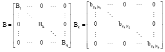 |
B is a q-block data-matrix, in which each block Bk has the main diagonal composed by the regression coefficients between the variable yk on xj, (j = 1, ..., p):
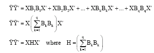
Then considering the pxq simple linear regressions, we run the prediction values Ŷ (Merola and Abraham, 2000; Ambra et al., 2001) and store them in a data-matrix:
| (6) |
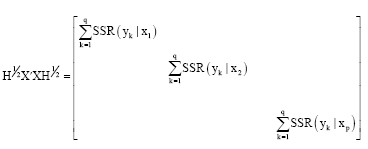
In computing the PCA of Ŷ and observing the matrix to diagonalize we develop the following expressions:
 | (7) |
They allow us to show as this approach could be viewed as a PCA of the prediction data matrix X with a particular metric expressed by a diagonal positive-definite matrix H½. The jth term of the main diagonal of this matrix represents a measure of the importance of the predictor xj (j = 1, ..., p) to explain all the dependent variables. This information could be used in order to choose the prediction variables to include in the model.
Hence, it is possible to consider this technique as a weighted PCA of X with weights proportional to the simple linear regression coefficients: we call it Multivariate Simple Linear Regression (MSLR). This approach could be seen as a generalization of the univariate PLS proposed by Garthwaite (1994).
If we take into account the matrix to diagonalize in the variable space, we can write it in term of Sum Square Regression (SSR) of the y on each x, infact we have:
 |
We, can underline as:
this expression allows us to say that the sum SSR between each yk (k = 1,..., q) on each xj = (j = 1, ..., p) is equal to the sum of the eigenvalues. If the variables are assumed standardized, every SSR can be interpreted as a determination coefficient (R2).
We can study MSLR results in the space of the variables and statistical units. In particular the coordinates of the statistical units and the variables on the alphath axis are:
| (8) |
where, uα and vα are the eigenvectors corresponding to the alphath eigenvalue. If we construct the factorial plan with the representation of predictor and dependent variables, we can compare the angle between variables in order to evaluate their relationship.
It’s possible to show that the principal components φα could be obtained as the minimization of the criterion:
where, ![]() is the simple orthogonal projector-operator.
is the simple orthogonal projector-operator.
Simulation Studies
The Simulation Plan
The data system was composed by two artificial matrices X (predictor variables) and Y (dependent variables) with 10000 statistical units and six and five variables respectively. The simulation regards the X, particularly for each degree of correlation between the X’s variable 100 matrices were generated. We shall also assume data are standardized by subtracting means and dividing by the standard deviation.
The correlation degrees investigated between X’s variables were 13 (0; 0.1; 0.2; 0.3; 0.4; 0.5; 0.6; 0.7; 0.8; 0.9; 0.95; 0.99; 0.999); particular attention to high level was paid.
The simulated data of the X were generated according to Cholesky algorithm (Olkin, 1985). The different five statistical methods discussed above were applied to these data.
The same simulation scheme has been repeated five times and for each of them all the statistical methods were calculated.
For each method the estimated values were calculated (Table 1) and then they were stored in a data-matrix. A PCA was performed on the estimated values; in Table 1 we represented the operator, the characteristic equation and the Criterion to minimize for each method.
Then, we have taken into account the first two components that guaranteed a percentage of explicated variability greater than 70%. Next, to the purpose to measure the similarity among the results achieved with each method, the mean of RV coefficient (Escoufier, 1970) has been computed for each pair of methods in the five simulations.
The RV coefficient quantifies the similarity between two data-matrices. It is a measure of the relationship between two sets of variables and it is based on the principle that two sets of variables are perfectly correlated if there exists an orthogonal transformation that makes the two sets coincide.
Let X and Y be two matrices corresponding to two sets of variables defined for the same n statistical units. If X and Y are centered by columns, the RV coefficient is defined by:
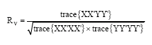 | (9) |
| Table 1: | Summary of the main characteristics of the statistical methods used in simulation study |
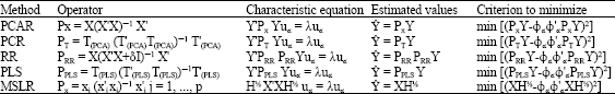 | |
The RV coefficient takes values between 0 and 1 for positive semi definite matrices. If we have a look at the numerator, it equals the sum of the square covariance (or correlation if the variables are scaled) between the variables of X and the variables of Y. It is therefore a square correlation coefficient.
This expression implies that RV(X, Y) = 1 if and only if the distance between the two data matrices is zero (d(X, Y) = 0).
RESULTS
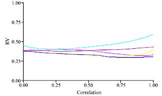
In order to compare the component based methods described above to each other and to MSLR we constructed a graphical representation of the five simulations. We represented the RV coefficient against different levels of correlation between X’s variables.
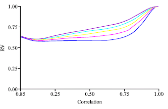
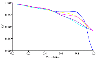
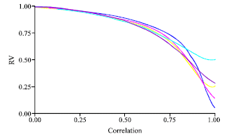
SLR-RIDGE had an RV coefficient that swells when the correlation between the X’s variables increases (Fig. 1); in particular, if correlation is greater than 0.90, the RV is very close to one (Fig. 2).
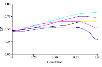 | |
| Fig. 1: | MSLR-RR (RV coefficient vs. correlation degree) |
 | |
| Fig. 2: | MSLR-RR (RV coefficient vs. correlation degree) |
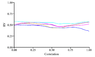
The relationship MSLR-RIDGE has been analysed varying the ridge parameter for five different values (0.2; 0.4; 0.6; 0.8; 0.9). We observed that when the correlation was smaller then 0,4 the RV coefficient was about 0,6, independently from the ridge parameter (Fig. 3).
Differently, when the correlation was included between 0.6 and 0.9, the behaviour of RV was a little bit different varying the ridge parameter. If the correlation was very close to one (r>0.98), the RV focused to one independently from the ridge parameter (Fig. 3).
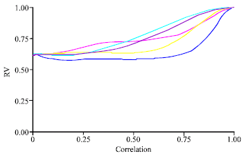
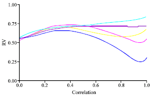
MSLR seemed less and less similar to both PCAR and PLS, when the correlation increased. Particularly, when the correlation between X’s variable was low the RV value for the three methods was about 0.50 (Fig. 4, 5).
 | |
| Fig. 3: | MSLR-RR(1) (RV coefficient vs. correlation degree) |
 | |
| Fig. 4: | PCAR-MSLR (RV coefficient vs. correlation degree) |
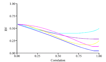 | |
| Fig. 5: | MSLR-PLS (RV coefficient vs. correlation degree) |
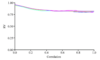
PCAR and PLS were very similar (RV>0.80) for whatever correlation value, however the trend decreases (Fig. 6).
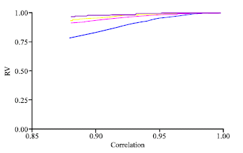
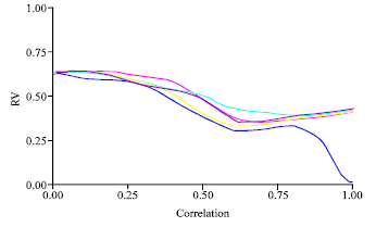
The similarity between RIDGE-PLS fell off when the correlation increased (Fig. 7). PCAR-RIDGE were similar when the correlation between X’s variable was low (r<0.5). Then the methodologies became very different (Fig. 7, 8).
The PCR had a likeness medium with the other methodologies (PLS-SLR-ACPR-RIDGE), independently from the correlation level between X’s variables (Fig. 9-12).
 | |
| Fig. 6: | PCAR-PLS (RV coefficient vs. correlation degree) |
 | |
| Fig. 7: | RR-PLS (RV coefficient vs. correlation degree) |
 | |
| Fig. 8: | PCAR-RR (RV coefficient vs. correlation degree) |
 | |
| Fig. 9: | PCR-PLS (RV coefficient vs. correlation degree) |
 | |
| Fig. 10: | MSLR-PCR (RV coefficient vs. correlation degree) |
 | |
| Fig. 11: | PCAR-PCR (RV coefficient vs. correlation degree) |
 | |
| Fig. 12: | PCR-RR (RV coefficient vs. correlation degree) |
CONCLUSION
In this study we have considered the problem of the multicollinearity in the analysis of dependence between two sets of variables defined for the same statistical units. In particular, we compared the main methods recommended in literature to counter this problem and proposed a new approach called MSLR. In order to evaluate the behaviour of these methods we have performed a simulation study, in which we can remark: in the first place, PCR shows a middle similarity with all the other methods, probably because it transforms the X variables in an orthonormal basis of variables eliminating the collinearity between predictor variables.
Secondly, considering the situation where the collinearity of X variables is almost 0.9 (very high collinearity) we have observed that MSLR is very similar to RR, independently from the ridge parameter. This characteristic allows to consider MSLR as a possible solution to use in presence of multicollinearity. Moreover, as shown in the previous paragraph, MSLR supplies in addition a very useful and simple interpretation of the estimated coefficients and the graphics.
REFERENCES
- Abdi, H., 2003. Partial Least Squares Regression (PLS regression). In: Encyclopedia for Research Methods for the Social Sciences, Lewis-Beck, M., A. Bryman and T. Futing (Eds.). Thousand Oaks (CA), Sage, pp: 1-7.
Direct Link - Carrol, J.D., 1968. Generalization of canonical correlation analysis to three or more sets of variables. Procesding of the 76th Annual Convention of the American Psychology Assocciation, (ACAPA'68), Washington DC., pp: 1-757.
Direct Link - Filzmoser, P. and C. Croux, 2002. A Projection Algorithm for Regression with Collinearity. In: Classification, Clustering and Data Analysis, Jajuga, K., A. Sokolowski and H. Bock (Eds.). Springer-Verlag, Berlin, Germany, ISBN: 978-3-540-43691-1, pp: 227-234.
Direct Link - Frank, I.E. and J.H. Friedman, 1993. A statistical view of chemometrics regression tools. Technometrics, 35: 109-148.
Direct Link - Garthwaite, P.H., 1994. An interpretation of partial least squares. J. Am. Stat. Assoc., 89: 122-127.
Direct Link - Helland, I.S., 1990. PLS regression and statistical models. Scandivian J. Stat., 17: 97-114.
Direct Link - Helland, I.S. and T. Almoy, 1994. Comparison of prediction methods when only a few components are relevant. J. Am. Stat. Assoc., 89: 583-591.
Direct Link - Hocking, R.R., 1996. Methods and Applications of Linear Models: Regression on and the Analysis of Variance. 1st Edn., John Wiley and Sons, London, ISBN-10: 047159282X, pp: 731.
Direct Link - Hoerl, A.E. and R.W. Kennard, 1970. Ridge regression: Biased estimation for nonorthogonal problems. Technometrics, 12: 55-67.
CrossRefDirect Link - Jolliffe, I.T., 1982. A note on the use of principal components in regression. Applied Stat., 31: 300-303.
Direct Link - Kattering, H., 1971. Canonical analysis of several sets of variables. Biometrka, 58: 433-451.
CrossRefDirect Link - Massy, W.F., 1965. Principal components regression in exploratory statistical research. J. Am. Stat. Assoc., 60: 234-256.
Direct Link - Naes, T. and I.S. Helland, 1993. Relevant components in regression. Scandivian J. Stat., 20: 239-250.
Direct Link - Stone, M., R.J. Brooks, T. Fearn, M. Denham and A.C. Atkinson et al., 1990. Continuum regression: Cross-validated sequentially constructed prediction embracing ordinary least squares, partial least squares and principal components regression. J. R. Stat. Soc., 52: 237-269.
Direct Link