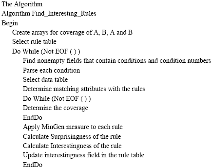
INTRODUCTION
A data mining technique usually generates a large amount of patterns and rules. However, most of these patterns are not interesting from a users point of view. Beneficial and interesting rules should be selected among those generated rules. This selection process is what we may call a second level of data mining; mining among rules. A pattern is interesting if it is easily understood, unexpected, potentially useful and actionable, novel, or it validates some hypothesis that a user seeks to confirm.
Systems that learn from examples often express the learned concept as a disjunction. The size of a disjunct is defined as the number of training examples that it correctly classifies (Holte et al., 1989). A number of empirical studies have demonstrated that learned concepts include disjuncts that span a large range of disjunct sizes and that the small disjuncts-those disjuncts that correctly classify only a few training examples-collectively cover a significant percentage of the test examples (Holte et al., 1989; Ting, 1994; Weiss and Provost, 2003). It has also been shown that small disjuncts often correspond to rare cases within the domain under study (Weiss and Provost, 1995) and cannot be totally eliminated if high predictive accuracy is to be achieved (Holte et al., 1989).
The very important reason to learn to deal with the two types of disjuncts
differently when comes the issue of interestingness of the disjuncts is that
there is the strong need to build machine learning programs which can improve
the accuracy of small disjuncts without significantly decreasing the accuracy
of the large disjuncts, so that the overall accuracy of the learned concept
is improved. Several researchers have attempted to build such learners. One
approach involves employing a maximum specificity bias for learning small disjuncts,
while continuing to use the more common maximum generality bias for the large
disjuncts (Holte et al., 1989; Ting, 1994). Unfortunately, these efforts
have produced, at best only marginal improvements. As they deal with only the
accuracy part of the rule interestingness. It is worth noting that the rule
interestingness comprises both the accuracy and surprisingness of the rule.
In this study we use MinGen measure given by Freitas (1998) which was originally proposed for small disjuncts; along with applying the Piateesky-Shapiro (1991) maximum generality bias measure for large disjuncts and Tan, 2000) maximum specificity bias measure for small disjunct. So trying to completely cover the issue of rule interestingness with this study.
BACKGROUND
A classification rule is a knowledge representation of the form A→B, where
A is a conjunction of predicting attribute values and B is the predicted class.
When evaluating the quality of a rule, three common factors to be taken into
account are the coverage, the completeness and the confidence factor of the
rule, defined as follows. The coverage of the rule (i.e., the number of tuples
satisfied by the rule antecedent) is given by |A|. The rules completeness (or
proportion of tuples of the target class covered by the rule) is given by |A
and B|/|B|. The rules confidence factor (or predictive accuracy) is given by
|A and B|/|A|. Piatetsky-Shapiro (1991) has proposed three principles for rule
interestingness (RI) measures, as follows.
• |
RI = 0 if |A and B| = |A| |B|/N.
|
• |
RI monotonically increases with |A and B| when other parameters are fixed.
|
• |
RI monotonically decreases with |A| or |B| when other parameters are fixed.
|
The first principle says that the RI measure is zero if the antecedent and the consequent of the rule are statistically independent. The second and third principles have a more subtle interpretation. Note Piatetsky-Shapiro (1991) was careful to state these principles in terms of other parameters, which is a phrase general enough to include any other parameter that we can think of. Let us assume for now that the rule parameters referred to by these principles are the terms |A|, |B| and |A and B|, which are the terms explicitly used to state the principle. Note that this is an implicit assumption in most of the literature. However, we will revisit this assumption later in this section. With the above assumption, principle 2 means that, for fixed |A| and fixed |B|, RI monotonically increases with |A and B|. In terms of the above mentioned rule quality factors, for fixed |A| and fixed |B|, the confidence factor and the completeness of the rule monotonically increase with |A andB| and the higher these factors the more interesting the rule is.
Principle 3 means that: (1) for fixed |A| and fixed |A and B| (which implies a fixed coverage and a fixed confidence factor) RI monotonically decreases with |B|-i.e., the less complete, the less interesting the rule is and (2) for fixed |B| and |A and B| (which implies a fixed rule completeness) RI monotonically decreases with |A| - i.e., the greater the coverage, the smaller the confidence factor and the less interesting the rule is.
Major and Mangano (1993) have proposed a fourth principle for RI measures (which
does not follow from the first three principles), namely:
• |
RI monotonically increases with |A| (rule coverage), given
a fixed confidence factor greater than the baseline confidence factor (i.e.,
the prior probability of the class). It should be noted that the above principles
were designed mainly for considering the widely-used rule quality factors
of coverage, completeness and confidence factor.
|
Another widely-used rule quality factor is rule complexity. Although these factors are indeed important when evaluating the quality of a rule, they are by no means the only ones. In this study we draw attention to five other factors related to rule quality and particularly to rule interestingness. These additional factors are discussed in the next subsections.
Note that, in theory, Piatetsky-Shapiros principles still apply to rule interestingness measures considering these additional factors, as long as they remain fixed. (As mentioned before, the principles were carefully defined with the expression fixed other parameters.) The problem is that, in practice, these additional factors do not remain fixed. These additional factors will probably vary a great deal across different rules and this variation should be taken into account by the rule interestingness measure.
OUR APPROACH
As we have stated that issue of interestingness of the discovered rules, whether the data mining task is association analysis or classification, is as important from the decision makers point of view as the any other step involved in the complete data mining process. There are several factors that should be considered while determining the interestingness of the generated rules. Here it is discussed how these factors should be evaluated and integrated into the rule selection mechanism. For this reason, we present a step-by step schema to produce really interesting rules.
Misclassification Costs
We have seen that misclassification costs are important for rule interestingness.
A rule predicting a patient does not have a particular disease while he indeed
does is very risky and misclassification cost of such a rule is very high. In
domains where we cannot tolerate erroneous classifications, a rule which has
a low error rate and low misclassification cost is more desirable.
In order to integrate this inverse proportion to the rule interestingness calculations,
we should divide the basic rule interestingness measure by the misclassification
cost of the rule, which is defined as follows:
Here Prob (j) is the probability that a tuple classified by the rule has true
class j, class I is the class predicted by the rule and cost (I, j) is the cost
of misclassifying a tuple with true class j as class I and k is the number of
classes. Prob (j) can be calculated as follows, taking into account the effect
of disjunct size:
Suppose there are two classes for the goal attribute, then k takes the value
2 and the formulae becomes
We are not assigning misclassification costs as we are trying to simply apply the rule interestingness measure on the generated rules, but if these rules are used for some specific applications like acceptance of credit or loan request on the basis of income level then the misclassification cost must be applied. In order for that cost matrix must be built, according to some expert of that domain.
The MinGen measure
Freitas (1998) has proposed a new measure which is very specific to the
classification rule discovery. This measure was originally proposed in the context
of small disjuncts. Formula given by Freitas considers the minimum generalizations
of the current rule r and counts how many of those generalized rules predict
a class different from the original rule r. Let m be the number of conditions
(attribute-value pairs) in the antecedent part of the rule r. Then rule r has
m minimum generalizations. The kth minimum generalization of r, k
= 1,........,m is obtained by removing the kth condition from r.
Let C be the class predicted by the original rule r (the majority class among
the examples covered by the antecedent of r) and Ck be the class
predicted by the kth minimum generalization of r (the majority class
of the examples covered by the antecedent of the k-th minimum generalization
of r). The system compares C with each Ck, k = 1,.....,m and N is
defined as the number of times where C is different from Ck.
The number N, in the range 0 to m could be defined as the degree of surprisingness of rule r-the larger the value of N the more surprising rule r is, in the sense of predicting a class different from its minimum generalizations.
Each of the m generalized rules produced by this procedure covers a superset of the examples covered by the original, specific rule r. As a result the distribution of the classes in the set of examples covered by each generalized rule can be significantly different from the distribution of the classes in the rule r. Hence the rule consequent (predicted class) is recomputed for each generalized rules will predict the most frequent class in its set of examples.
However, that measure would be biased to favor very long rules (with many conditions),
i.e., the value of the measure would tend to grow with the value of m. In order
to avoid a potential confusion, the following normalized version of the rule
surprisingness measure, denoted by MinGen:
The larger the value of this measure, the more surprising the rule is. One disadvantage of this rule surprisingness measure is its relatively high computational cost. For each specific rule being evaluated, the system needs to compute m generalized rules.
Finding Interesting Rules In US. Census Data
In this study, the rule interestingness measure mentioned above is applied
to US Census data collected from the UCI repository. This data was extracted
from the census bureau database found at| http://www.census.gov/ftp/pub/DES/www/welcome.html|
Domain Description
In our experimentation domain, we are trying to predict whether an individuals
total income is less than or greater than $50,000$ by looking at some information
about the individual. Prediction task is to determine the income level for the
person represented by the record. The data was split into train/test in approximately
2/3, 1/3. There are 40 attributes in the census database and Incomes have been
binned at the $50K level to present a binary classification problem. For our
experimentation we have selected education, major occupation code and income
attributes to simplify the matters.
Basic statistics for this data set:
Number of instances data = 199522
17 distinct values for attribute education nominal
15 distinct values for attribute major occupation code nominal
There is the database table occupation.txt which consists of the above mentioned
attributes. After applying the Christian Borgelts rule induction program on
this Table 1 17 rules are generated by taking the default
parameters.
No. of records containing income $+50,000 = 3392
No. of records containing income $-50,000 =196130
Persons having income less than $50,000 are in class -50,000 and persons having
income greater than $50,000 are in the class +50,000. So, this reduces to a
binary classification problem.
Experimental Details
In our domain, the attributes have no acquirement costs since they are mostly
demographic information. Also, they are not given weights, since all attribute
are of the same interest. We are not interested in particularly identifying
any one class, we do not assign weights to classes either. Since class +50,000
is the minority class in the dataset and rules predicting the minority class
are already counted as more interesting, assignment of weights to classes is
not essential in our example domain.
Grouping by Coverage Values
It is clear from various studies that small and large disjuncts; i.e., the rules
having low coverage (support) and rules having large coverage should be evaluated
in different ways. For this evaluation, Holte et al. (1989) suggested
that small disjuncts should be evaluated with a maximum-specificity bias, in
contrast with the maximum-generality bias favoring large disjuncts. Tan and
Kumar also argued that a good interestingness measure should take into account
the support of the pattern. They have showed that their proposed IS measure
can be used in the region of low support, i.e., support of 0.3, whereas using
RI measure in the region of high support is preferred. Hence, in order to make
small disjuncts as interesting as large disjuncts, IS measure may be taken as
the basic measure for rules having coverage values in the range of (0,0.3) and
RI measure for rules with coverage values (0.3,1). Here are the formulations
for two measures, respectively:
MinGen measure (Freitas, 1998) must be applied to rule interestingness calculation of classification rules for surprisingness factor to be taken into account.
Experimental Results
Borgelts (1997) rule induction algorithm is applied to the database. Total
117 rules are generated as a result of the rule generator program. Confidence
level pruning is done. USCensus database is being classified for the income
level less than or greater than 50K $ on the basis of education level and occupation
code.
In the first run all rules were evaluated on the basis of RI measure and then in the second run small disjuncts are evaluated on the basis of IS measure and large disjuncts are evaluated on the basis of RI measure. Thus we calculate the accuracy of each rule applying different biases for small and large disjuncts.
After applying the MinGen measure to rules we get the values of surprisingness for the rules. It is obvious that Interestingness = Accuracy + Surprisingness
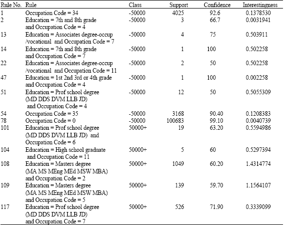
Now we can finally state the exact interestingness of the rules as shown in the Table 1.
In Table 1, one important observation is that the most interesting
rule is the one belonging to class 0 and also in the rest of the list, rules
belonging this class are in higher levels to.
Table 1: |
Interestingness values with MinGen measure |
 |
CONCLUSION AND FUTURE WORK
This research provides insight into the degree of variation according to the disjunct size in learning. By measuring interestingness of rules induced from US Census database, we demonstrated that some domains are prone to the problem of small disjuncts and class skews and accordingly the measure of interestingness must be chosen to deal with them.
Although the focus of this study was on measuring the interestingness of discovered rules and understanding the impact of small disjuncts on learning, present results could lead to improved learning algorithms.
We believe that the special contribution of this study is to gain attention towards applying not only different learning biases for rules but also to adopt some specific measure for rule surprisingness as this is the inseparable part of rule interestingness along with the rule accuracy.
For future research, by taking into account different conditions (attributes), further researches can be performed. Another possible research area can be to apply the classification analysis in this domain for some real world applications and accordingly different factors affecting the rules interestingness like misclassification cost, attribute usefulness and class weights can be determined with the help of domain experts. The most important study is to show the results to the user of the domain and accordingly rules real interestingness can be determined.