
Ashutosh Bagchi
Department of Building, Civil and Environmental Engineering, Concordia University, Montreal, Quebec, 1455 de Maisonneuve Blvd. West, H3G 1M8, Canada
Trends in Applied Sciences Research
Year: 2012 | Volume: 7 | Issue: 3 | Page No.: 196-209


ABSTRACT
Thin shells are prone to fail by buckling due to compressive membrane stress. Although shells develop primarily membrane stresses, in most practical situations, they have some bending stresses as well as a result of supports, loading condition and discontinuity. In such case, the response of a shell to external loads becomes nonlinear. Linearization of the nonlinear equilibrium equations gives rise to an eigen value problem solving which buckling load is obtained. Eigen value buckling analysis is computationally faster than the nonlinear analysis involving tracing the load-deflection path and finding the corresponding collapse load. However, the buckling load estimated using the eigenvalue buckling analysis is approximate and usually overestimated. For the systems with large prebuckling rotations this approach may give highly unconservative results. Attempts have been made for better prediction of actual buckling load of shells of revolutions by combining eigenvalue buckling analysis and geometric nonlinear analysis. Such methods are computationally more efficient than the nonlinear buckling analysis but more reliable than the linear buckling analysis. This study presents an overview of the stability analysis of shells of revolution using a conical frustum shell element incorporating the linear and simplified nonlinear buckling analysis including the treatment of initial geometric imperfection.
PDF Abstract XML References Citation
Received: November 04, 2011;
Accepted: February 02, 2012;
Published: February 25, 2012
How to cite this article
Ashutosh Bagchi, 2012. Linear and Nonlinear Buckling of Thin Shells of Revolution. Trends in Applied Sciences Research, 7: 196-209.
URL: https://scialert.net/abstract/?doi=tasr.2012.196.209
URL: https://scialert.net/abstract/?doi=tasr.2012.196.209
INTRODUCTION
Thin shells and plates are very common in structural constructions. In the design of thin shells (or plates) buckling is an important factor to be considered. Buckling may be overall (global) or local. Buckling of axisymmetric shells, especially cylinders, received a good amount of attention in the past (Timoshenko and Gere, 1963; Bushnell, 1985; Al-Qablan, 2010). A lot of theoretical work to predict the buckling load of these structures is available in the literature. With finite element method, it is possible to analyze more complex shells and other structures (Wood and Zienkiewicz, 1977; Boumechra and Kerdal, 2006; Bagchi et al., 2007; El-Kafrawy and Bagchi, 2007). An insight on the local buckling of axisymmetric shells has been provided by Cai et al. (2002), while Athiannan and Palaninathan (2004) presented an experimental evaluation of stability of shells of revolution under axial and shear stresses. Jasion (2009) conducted linear buckling and nonlinear post-buckling analysis of shells of revolution under external pressure and determined that convex barrel shape shells are not stable in the postbuckling regime. Bochkarev and Matveenko (2011) studied the dynamic and stability behavior of shells of revolution under internal fluid pressure. Ummenhofer and Knoedel (2000) studied the effect of boundary condition on the behavior of steel cylindrical shells under wind load. The initial geometric imperfection that may be present in a shell reduces the buckling capacity. There are some experimental and analytical works on shells of revolution with geometric imperfection available in the literature (Freskakis, 1970; Freskakis and Morris, 1972; Frano and Forasassi, 2008). Abdullah et al. (2008) studied the fatigue life of shells with variable amplitude loading, while Khamlichi et al. (2010) and Bahaoui et al. (2010) explored the effect of localized interacting defects on the critical loads for cylindrical shells under compression. Thermal effect of the stability of axisymmetric shells has been reported in the literature (Bagchi and Paramasivam, 1995; Sheng and Wang, 2010; Ghorbanpour, 2002).
In the finite element context, there are two types of buckling analysis methods normally used, linear and nonlinear. Linear buckling analysis is also called eigenvalue buckling analysis because, it gives rise to an algebraic eigenvalue problem. This method has two versions, classical and fully linearized buckling analysis. Linear buckling analysis gives good prediction of buckling load of a structure if the prebuckling rotations are negligible. However, in practice, shell structures have considerable prebuckling rotations and linear or eigenvalue buckling analysis alone is not sufficient to predict the stability limit of these structures. Full nonlinear analysis would give the exact estimate of collapse load in those cases. But full nonlinear analysis is very costly and time consuming when the size of the structural model is large.
An improved method for prediction of buckling load was suggested by Brendel and Ramm (1980). The linear stability analysis usually performed for initial position was repeated at different load levels on the nonlinear prebuckling path. Thus a current estimate of the final failure load was obtained and using this information the so called eigenvalue function was traced. They used the characteristics of the eigenvalue function in predicting the nonlinear buckling load. Based on this methodology Chang and Chen (1986) proposed a scheme for predicting actual buckling load of a structure by properly combining linear buckling analysis and geometrically nonlinear prebuckling analysis with minimum number of load steps. They have implemented the method for beams and general shell elements and demonstrated the effectiveness of the method by some numerical experiments.
The simplified nonlinear buckling analysis procedure developed by Chang and Chen (1986) for shells of revolution was extended by Bagchi and Paramasivam (1996). The method was implemented by using conical shell element with four degree of freedom (d.o.f) per node (Navaratna et al., 1968) as shown in Fig. 1 which was initially extended to solve for thermal stress and buckling capacity of shells of revolution (Paramasivam et al., 1995; Bagchi and Paramasivam, 1995) The basic philosophy of this method is that critical load obtained by eigenvalue buckling analysis based on stressed structure under a certain load level, in most of the cases, will be closer to the actual stability limit than that obtained from an unstressed structure.
 | |
| Fig. 1: | The conical frustum shell (CFS) element |
This method can be used to determine the bifurcation point (where the load deflection curve deviates from the primary path), if that exists. The present article provides an overview of the stability analysis of axisymmetric shells with implementation of the linear and simplified nonlinear buckling analysis procedure mentioned earlier including the effect of initial geometric imperfection.
THE AXISYMMETRIC SHELL ELEMENT
A conical frustum shell element (Fig. 1) is used for the present analysis. The element has two nodal circles (i and j) and four degrees of freedom (d.o.f.) at each nodal circle. The d.o.f.s correspond to meridional displacement (ui and uj), circumferential displacement (vi and vj), normal displacement (wi and wj) and meridional rotation (βi and βj). There are three components of the field displacement, u, v and w; where, u and v are linear functions and w is a cubic function. The displacement functions are expressed in terms of the nodal d.o.f.s and Fourier harmonics, n (to represent the circumferential variation). L is the length of the element, s is the coordinate along L and ξ = s/L (a non dimensional coordinate):
 | (1) |
The field displacements u, v and w can be expressed in terms of the element degrees of freedom using appropriate shape functions as shown in Eq. 2:
 | (2) |
LINEAR BUCKLING ANALYSIS
In most shell structures, prebuckling stresses consist of both membrane stresses and bending stresses and the problem basically becomes nonlinear in terms of load and displacements. Because of this fact it is more realistic to find the nonlinear response of the structure by step by step incremental iterative method which is an expensive and time consuming procedure. Linear buckling analysis is comparatively very efficient but the results obtained by this method should be interpreted carefully.
The strain-displacement relation of a structural element in the discretized form can be written as ε = Bδ, where B is the strain matrix. B matrix can be broken into two, part is contributed by the linear part of the strain and the other part is contributed by the higher order terms in the generalized strain expression. Considering the generalized strain-displacement up to the quadratic term B matrix can be expressed in the following form (Wood and Zienkiewicz, 1977):
| (3) |
Differentiating the expression in Eq. 3 with respect to δ, we can obtain the strain-displacement relationship in the incremental form as shown in Eq. 4:
| (4) |
Then equilibrium equation in the incremental form can be expressed as in Eq. 5:
| (5) |
The solution of Eq. 4 can be approached iteratively, using methods such as, the Newton-Raphson (NR) method or its modified version. Taking appropriate variation of Eq. 6 with respect to δ we have:
| (6) |
where, KT is the tangent stiffness matrix which can be expressed as the sum of K0, the initial stiffness, KL, the stiffness contribution due to geometric nonlinearlity or the second order strain as shown in Eq. 2 and Kσ, the stiffness due to axial stress or the geometric stiffness, as shown in Eq. 7. The expression for each of these stiffness terms are shown in Eq. 8:
| (7) |
 | (8) |
In Eq. 8, ![]() is a matrix of axial stress resultants and G represents a relation between the radial displacements to the axial strain. D represents the constitutive matrix. The stress-strain relationship is given by Eq. 9, where, N’s are the in-plane stress resultants, M’s are the moments and í is the Poisson’s ratio (assuming the material to be isotropic):
is a matrix of axial stress resultants and G represents a relation between the radial displacements to the axial strain. D represents the constitutive matrix. The stress-strain relationship is given by Eq. 9, where, N’s are the in-plane stress resultants, M’s are the moments and í is the Poisson’s ratio (assuming the material to be isotropic):
 | (9) |
The tangent stiffness matrix becomes singular (i.e., the determinant of the matrix becomes equal or very near to zero) at the critical load level, indicating that the load vector would cause the displacements to increase towards infinity. Let us assume that any arbitrary reference load is applied to the structure and it deforms to a state described by δ. In linear buckling analysis it is assumed that the incremental stiffness is a linear function of the displacements. Therefore, a positive constant λ, the structural deformation is described as λ δ for the applied load vector δP. When the critical load level is reached, the following eigenvalue equation (Eq. 10) is satisfied:
| (10) |
This algebraic eigenvalue problem can be solved by any standard algorithm. The lowest eigenvalue gives the critical buckling load factor and corresponding eigenvector describes the buckling mode. This formulation is called fully linearized buckling analysis. If the pre-buckling rotations are zero or negligible KL in Eq. 11 may be removed and the eigenvalue problem reduces to Eq. 9 which is called classical buckling analysis:
| (11) |
In buckling analysis of axisymmetric shells, the stiffness matrices are formed for various a number of Fourier harmonics, n and the eigenvalues are extracted corresponding to each harmonic. The lowest eigenvalue corresponds to the critical load. Derivation of the geometric stiffness matrix for the Conical Frustum Shell (CFS) element is described in the following paragraphs.
To obtain the initial stiffness K0, the small stress strain relation (Eq. 12) is considered, while for the geometric stiffness matrix Kσ and the large deflection stiffness matrix KL, the strains due to large displacements (Eq. 13) are required to be considered:
 | (12) |
 | (13) |
The element geometric stiffness matrices thus obtained are transformed and assembled in the global geometric stiffness matrix and the eigenvalue problem is solved for classical buckling analysis. For fully linearized buckling analysis KL matrix is also included.
INITIAL GEOMETRIC IMPERFECTION
Initial imperfection in a structure can be treated as initial displacements in the structure causing some initial strains. In that case the complete strain field for a structural element can be expressed as:
| (14) |
where, ![]() is the normal component of initial imperfection in the geometry of the shell (assuming that the imperfection is predominantly in the normal direction, not in other two directions). It is assumed that the circumferential variation is proportional to the buckling mode shape and can be expressed in terms of Fourier series in case the buckling mode shape is unsymmetric.
is the normal component of initial imperfection in the geometry of the shell (assuming that the imperfection is predominantly in the normal direction, not in other two directions). It is assumed that the circumferential variation is proportional to the buckling mode shape and can be expressed in terms of Fourier series in case the buckling mode shape is unsymmetric.
NONLINEAR BUCKLING ANALYSIS
Linear eigenvalue buckling formulation may also be applied to structures having a nonlinear prebuckling path with a bifurcation or limit point. In this case the lowest eigenvalue is more or less satisfactory estimate of the ultimate load. This eigenvalue analysis can be repeated for different load levels producing an estimate of the buckling load in an advanced position. If the function of the lowest eigenvalue is monitored parallel to the nonlinear load-deflection path it gives an indication of the distance between the critical load and the load level reached. Finally the eigenvalue function (also called the predicted-load curve (Chang and Chen, 1986) intersects the load deflection curve in the critical point (Brendel and Ramm, 1980) as shown in Fig. 2.
From previous discussions it is clear that the linear (classical and fully linearized) buckling analysis alone cannot give very useful prediction about the actual critical load of the structure. To improve the the approximation linear buckling analysis based on a stressed structure under a certain load level Pbase may be performed (Chang and Chen, 1986). The buckling load so obtained in most of the cases will be closer to the actual stability limit than that obtained from an unstressed structure.
To perform this type of analysis, the base load level, Pbase is first applied in increments or single step and a conventional nonlinear analysis using Newton-Raphson method is performed. The tangent stiffness matrix, KT corresponding to that equilibrium state is formed and as a succeeding step a trial load increment is applied and based on the incremental stresses and displacements Kσ and KL are formed.
 | |
| Fig. 2(a-b): | Scheme for simplified nonlinear buckling analysis: (a) the predicted load curve and (b) determination of the collapse load |
At this stage the eigenvalue problem is solved to find the proper load level beyond the fundamental load level, Pbase at which the tangent stiffness matrix of the structure becomes singular. If the critical load factors are plotted against the base load factors upon which the eigenvalue extraction are performed, Pbase in the predicted-load curve (same as eigenvalue function on P-V curve) will always terminate at the point of coordinate (Pcr, Pcr).
The combined nonlinear and linear buckling analysis outlined above can be applied with either the fully linearized or classical buckling analysis. First, a linear buckling analysis on a unstressed structure is performed and an approximate critical load, Pcr1 is obtained; then, at certain base load level Pbase another linear buckling analysis is performed to obtain a new prediction of buckling load, Pcr2. Finally, on a (Pbase-Pcr) graph (Fig. 2b), extrapolation from point (0, Pcr1) and (Pbase, Pcr2) is made to find its intersection with the 45° line. This approach for critical load prediction requires significantly less computation than that for conventional geometrically nonlinear analysis. It may provide a suitable guideline for applying load increments when a load-deflection curve is required to be traced. This procedure referred to as simplified or Quasi Nonlinear Buckling Analysis (QNBA) method by Bagchi and Paramasivam (1996).
NUMERICAL EXAMPLES
Truncated hemispherical shell subjected to axial tension: This is an interesting problem. The geometry and loading are as shown in Fig. 3. Under the action of axial tension, compressive stress develops in the hoop direction. This compressive hoop stress leads to buckling of the shell. This problem was originally reported by Yao (1963). He has presented experimental as well as theoretical results. His theoretical analysis was based on Galarkin's approach. Yao found a considerable discrepancy between theoretical and experimental buckling loads. The present analysis supports the theoretical value of critical load obtained by Yao (1963). Fully Linearized Buckling (FLB) analysis improves the result to a large extent. If the effect of imperfection is considered the value of buckling load obtained here is comparable to the experimental result. The values of different critical loads and number of circumferential waves are given in Table 1.
The truncated hemispherical shell problem (Fig. 3) is solved considering initial geometric imperfection and it is found that if the maximum deviation of the shell surface from the perfect geometry is equal to 0.4 times the thickness of the shell, the buckling load is 11.73x10⁻⁴ N/m (n = 40). This value is comparable to the experimental value of the buckling load reported by Yao (1963) which is 10.76x10⁻⁴ N/m (n = 39) (Table 1). The classical buckling mode shape is presented in Fig. 4.
 | |
| Fig. 3: | Truncated hemispherical shell under tension |
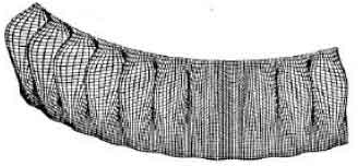 | |
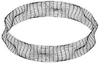
| Fig. 4: | Buckled shape of the truncated hemisphere (only a 45° segment is shown) |
 | |
| Fig. 5: | Axially loaded cylinder |
| Table 1: | Buckling load of a truncated hemispherical shell under tension |
| *Values in the parenthesis indicates value of n. The critical load is in 104 lb/in | |
Cylinders under axial load: Buckling of cylinders received a lot of attention of the engineers because of the extraordinary discrepancies between the buckling loads obtained by theory and experiment. Buckling of cylinders is greatly influenced by initial geometric or load imperfection and residual stresses in it. Here, the behaviour of the perfect cylinders is discussed and the closed form solutions are used to check the results obtained by linear buckling analysis theory. For perfect cylinders with simply supported edges, classical solutions are available (Timoshenko and Gere, 1963).
Finite element analysis agrees well at the above mentioned points. Results of axially compressed cylinders (Fig. 5) with different L/R and t/R ratios are presented in Fig. 6 and Table 2, respectively. From these tables it is clear that L/R ratio has very little effect (unless the cylinder is very short or very long) on critical load compared to the t/R ratio. Buckled shape of an axially loaded simply supported cylinder with modulus of elasticity E = 2x10⁵ MPa, v = 0.3 and L/R = 0.4 is shown in Fig. 7 as an example.
A spherical shell with external pressure and initial geometric imperfection: A spherical shell with geometry as shown in Fig. 8 is considered. E = 2x10⁵ Mpa and v = 0.3. The shell is subjected external pressure.
 | |
| Fig. 6: | Critical load for axially loaded cylinders |
 | |
| Fig. 7: | Buckled shape of a typical axially loade |
 | |
| Fig. 8: | A spherical shell with geometric imperfection |
| Table 2: | Effect of R/t ratio on the critical load of axially loaded cylinders |
 | |
Initial geometric imperfection of the shell is considerd parallel to the buckling mode.For different values of ![]() /t and Pi/P0 ratios are shown in Fig. 9. Here,
/t and Pi/P0 ratios are shown in Fig. 9. Here, ![]() the amplitude of initial geometric imperfection with respect to the perfect meridian of the shell, t is the thickness of the shell, Pi is the buckling load for the imperfect shell and P0 is the buckling load for the perfect shell. Similar types of problems were studied by Freskakis (1970) and Freskakis and Morris (1972). Although he assumed different shape of imperfection, those results are also presented here as reference.
the amplitude of initial geometric imperfection with respect to the perfect meridian of the shell, t is the thickness of the shell, Pi is the buckling load for the imperfect shell and P0 is the buckling load for the perfect shell. Similar types of problems were studied by Freskakis (1970) and Freskakis and Morris (1972). Although he assumed different shape of imperfection, those results are also presented here as reference.
It is observed from Fig. 9 that the buckling load reduces with the magnitude of initial geometric imperfection and the rate of reduction in buckling load increases with the increase in the magnitude of imperfection.
Spherical cap subjected to axisymmetric ring load: The geometry of the spherical cap is shown in Fig. 10. Geometrically nonlinear analysis of this shell was presented by Wood and Zienkiewicz (1977). The limit load is obtained from the graph presented by them (Plim = 336.0 N) and is compared with the collapse load obtained using simplified nonlinear buckling procedure QNBA (Bagchi and Paramasivam, 1996) which is (Pcr* = 361.3 N) and found to be significantly close (deviation of QNBA result is about 7.5% from actual axisymmetric collapse load).
 | |
| Fig. 9: | Effect of geometric imperfection on the critical load of the spherical shell |
 | |
| Fig. 10: | A spherical cap with ring load |
 | |
| Fig. 11: | Effect of load ring diameter on the collapse load |
It should also be noted that, axisymmetric shell subjected to axisymmetric load may not show axisymmetric collapse. The present analysis method is applied for other buckling mode with different numbers of circumferential waves and a still lower value of buckling load is recorded. For non-axisymmetric buckling Pcr* = 272.3 N. Figure 11 shows the variation of the collapse load with the position of the ring load. As the ring diameter increases, the collapse load increases.
CONCLUSIONS
The study provides a review of buckling behaviour of shells of revolutions with a systematic development of the conical shell elements and detailed formulation including geometric imperfection. It also presents the analysis of a number of cylindrical and spherical shells and compares the experimental collapse loads with the numerical results whenever available and performs the sensitivity of length, radius or length on the buckling load as appropriate. It is found that the numerical results albeit slightly unconservative can provide a good idea about the actual collapse load and the simplified nonlinear buckling analysis produces a reliable estimate of collapse loads when prebuckling rotations are significant. However, further work is necessary to study the effectiveness of the QNBA method for axisymmetric shells with more sophisticated elements. Based on the work presented in this article, the following conclusions are made:
| • | The two-noded conical frustum shell element is found to be very efficient for stability analysis in spite of its inherent limitations in modelling curved meridians. In the case of a curved meridian, very small elements should be used. Curved elements are not studied in this study |
| • | The classical buckling analysis is faster than the fully linearized buckling analysis. But the classical buckling analysis gives good prediction of actual buckling load only in the case of structure with membrane stresses alone or with negligible bending stresses |
| • | The fully linearized buckling analysis gives lower buckling load than that obtained by the classical buckling analysis. But sometimes, it may also give very conservative result when prebuckling rotations are higher |
| • | Convergence of the critical buckling load obtained by the classical buckling analysis with increasing number of elements is from the top and the buckling load predicted by this method is always in the higher side and unconservative |
| • | The nonlinear buckling load prediction by the simplified nonlinear analysis is found to be straight forward and very much economical. It gives reasonably accurate estimate of the actual collapse load of a structure with minimum effort |
ACKNOWLEDGEMENT
Support of the Natural Sciences and Engineering Research Council of Canada (NSERC) is greatly appreciated.
REFERENCES
- Al-Qablan, H., 2010. Semi-analytical buckling analysis of stiffened sandwich plates. J. Applied Sci., 10: 2978-2988.
CrossRef - Abdullah, S., S.M. Beden, A.K. Ariffin and M.M. Rahman, 2008. Fatigue life assessment for metallic structure: A case study of shell structure under variable amplitude loading. J. Applied Sci., 8: 1622-1631.
CrossRefDirect Link - Athiannan, K. and R. Palaninathan, 2004. Experimental investigations on buckling of cylindrical shells under axial compression and transverse shear. Sadhana, 29: 93-115.
Direct Link - Bagchi, A. and V. Paramasivam, 1995. Static and stability analysis of the inner vessel of a fast breeder reactor. J. Nuclear Eng. Design, 158: 81-94.
CrossRef - Bagchi, A. and V. Paramasivam, 1996. Stability analysis of axi-symmetric thin shells. ASCE J. Eng. Mechan., 122: 278-281.
CrossRef - Bagchi, A., J. Humar and A. Noman, 2007. Development of a finite element system for vibration based damage identification in structures. J. Applied Sci., 7: 2404-2413.
CrossRefDirect Link - Boumechra, N. and D.E. Kerdal, 2006. The P-version finite element method using bezier-bernstein functions for frames, shells and solids. J. Applied Sci., 6: 2334-2357.
CrossRefDirect Link - Bochkarev, S.A. and V.P. Matveenko, 2011. Natural vibrations and stability of shells of revolution interacting with an internal fluid flow. J. Sound Vibr., 330: 3084-3101.
CrossRefDirect Link - Brendel, B. and E. Ramm, 1980. Linear and nonlinear stability analysis of cylindrical shells. Comput. Structures, 12: 549-558.
CrossRef - Cai, M., J. Mark, F.G. Holst and J.M. Rotter, 2002. Buckling strength of thin cylindrical shells under localized axial compression. Proceedings of the 15th ASCE Engineering Mechanics Conference, June 2-5, 2002, Columbia University, New York, pp: 1-8.
Direct Link - Chang, S.C. and J.J. Chen, 1986. Effectiveness of linear bifurcation analysis for predicting the nonlinear stability limits of structures. Int. J. Numerical Methods Eng., 23: 831-846.
CrossRef - Bahaoui, J.E., A. Khamlichi, L.E. Bakkali and A. Limam, 2010. Reliability assessment of buckling strength for compressed cylindrical shells with interacting localized geometric imperfections. Am. J. Eng. Applied Sci., 3: 620-628.
CrossRefDirect Link - El-Kafrawy, O. and A. Bagchi, 2007. Computer aided design and analysis of reinforced concrete frame buildings for seismic forces. Inform. Technol. J., 6: 798-808.
CrossRefDirect Link - Frano, R.L. and G. Forasassi, 2008. Buckling of imperfect thin cylindrical shell under lateral pressure. Sci. Technol. Nuclear Installations.
CrossRefDirect Link - Freskakis, G.N. and N.F. Morris, 1972. Axisymmetric buckling of initially imperfect spherical shells. ASCE J. Eng. Mechan., 98: 1115-1131.
Direct Link - Ghorbanpour, A., 2002. Critical temperature of short cylindrical shells based on imnproved stability equation. J. Applied Sci., 2: 448-452.
CrossRefDirect Link - Jasion, P., 2009. Stability analysis of shells of revolution under pressure conditions. Thin-Walled Struct., 47: 311-317.
CrossRefDirect Link - Khamlichi, A., J.E. Bahaoui, L.E. Bakkali, M. Bezzazi and A. Limam, 2010. Effect of two interacting localized defects on the critical load for thin cylindrical shells under axial compression. Am. J. Eng. Applied Sci., 3: 464-469.
CrossRefDirect Link - Navaratna, D.R., T.H H. Pian and E.A. Witmer, 1968. Stability analysis of shells of revolution by the finite element method. AIAA J., 6: 355-361.
Direct Link - Sheng, G.G. and X. Wang, 2010. Thermoelastic vibration and buckling analysis of functionally graded piezoelectric cylindrical shells. Applied Math. Modell., 34: 2630-2643.
CrossRef - Ummenhofer, T. and O. Knoedel, 2000. Modelling of boundary conditions for cylindrical steel structures in natural wind. Proceedings of the 4th International Colloquium on Computation of Shell and Spatial Structures, June 5-7, 2000, Chania, Crete, Greece, pp: 1-15.
Direct Link - Wood, R.D. and O.C. Zienkiewicz, 1977. Geometrically nonlinear finite element analysis of beams, frames, arches and axisymmetric shells. Comput. Structures, 7: 725-735.
CrossRef - Yao, J.C., 1963. Buckling of truncated hemisphere under axial tension. AIAA J., 1: 2316-2319.
Direct Link
Adeola A Adedeji Reply
A well articulated paper. Very interesting reading.....