
B. Bala Tripura Sundari
Amrita School of Engineering, Amrita Vishwa Vidyapeetham, 641112, Coimbatore, India
Journal of Artificial Intelligence
Year: 2012 | Volume: 5 | Issue: 4 | Page No.: 142-151


ABSTRACT
Recently, FPGA (Field Programmable Gate Arrays) technologies have made significant advances in both speed and capacity. Specifically, the design methodology to map the loop dependencies in a do loop algorithm on to a linear array of processors after extraction of parallelism is a challenging task. The mapping of Full Search Block Motion Estimation (FSBM) and edge detection algorithms are taken up here as they represent multi loop nested algorithms that are intensive in computations. Also, a method of prefixing the elements in the mapping vectors has been used which reduces the search space for both the algorithms. The formulation of a dependence vectors for the FSBM is explained and the architecture for the computationally intensive FSBM and Edge detection algorithm is developed and the simulation and synthesis results are presented.
PDF Abstract XML References Citation
Received: October 17, 2012;
Accepted: November 10, 2012;
Published: January 09, 2013
How to cite this article
B. Bala Tripura Sundari, 2012. Mapping Multi-Loop Nest Algorithms on to Reconfigurable Architecture. Journal of Artificial Intelligence, 5: 142-151.
DOI: 10.3923/jai.2012.142.151
URL: https://scialert.net/abstract/?doi=jai.2012.142.151
DOI: 10.3923/jai.2012.142.151
URL: https://scialert.net/abstract/?doi=jai.2012.142.151
INTRODUCTION
Nested loop algorithms represent the set of algorithms which are computationally intensive. They also exhibit inherent parallelism. Hardware implementation of these algorithms exploits this inherent parallelism to speed up the processing. The parallelism could be achieved by using array of Processing Elements (PEs) termed s systolic arrays to speed up computationally intensive applications (Kittitornkun and Hu, 2001; Yeo and Hu, 1995). Previously many methodologies have been proposed to map nested-loop algorithms onto linear array illustrates the method of deriving systolic arrays by obtaining the cut-set systolization process (Kung, 1985). A systematic approach for mapping parallel algorithms into 2D array is proposed using the concept of SA statements in (Al-Khalili, 1995). Linear array implementations of 2D matrix array have been shown in this study (Kumar and Tsai, 1991). Lee and Kedem (1988) proposed linear families of processing elements have for mapping depth P-nested for loop algorithms.
The mapping of the algorithm onto the array of processors is a challenging task. In addition to this, the appropriate flow of input data to the array of processors, the data reuse amongst array of processors to implement the various steps of the algorithm, the flow of the output data after the completion of the iteration are the multiple tasks to be addressed for a successful mapping.
The following two computationally intensive tasks of image processing algorithms are considered:
| • | The full search block motion estimation (FSBM algorithm) (Komarek and Pirsch, 1989) |
| • | Edge Detection (ED) algorithm |
MAPPING PROCESS
In this study, the focus is on image processing algorithms. Most of the image processing algorithms are computationally intensive and exhibit inherent parallelism. This parallelism can be exploited while implementing hardware architectures. The parallelism means that there will be common operations whose order of execution is not important for the final result. For example, in matrix-matrix multiplication the order in which we add the inner product to form a value in the result vector is not important. Similarly in FSBM algorithm, the order in which the MADs of individual blocks are compared is also unimportant.
Selection of PE count: In FSBM given in Listing 1, the image is divided into NhxNV sub-frames of size NxN pixels and p is the search direction parameter. The current frame pixels are represented by X and previous frame pixels by Y.
In some of the image processing algorithms like FSBM, edge detection etc., we can approximately determine the number of Processing Elements (PEs) beforehand. For example in FSBM a total of (2p+1)2 identical operations has to perform for each pixel in an image frame, where p is the search parameter. Similarly in edge detection algorithm each image pixel has to be multiplied by W2 window coefficients where the convolution mask size is WxW. So, it is convenient to begin with (2p+1)2 PEs in the former case and W2 PEs in the later case. This is also corroborated in the mapping algorithm. In this way we avoid the process of calculating the number of PEs, thereby speeding up the mapping process. We followed this approach in our mapping process for FSBM and ED algorithms.
Selection of number of ports: The architecture for FSBM algorithm as given in uses 4 ports which includes 2 ports for accessing the y frame data (Kittitornkun and Hu, 2001). We assume the number of ports required for the architecture by taking into the account the core functionality of a nested loop algorithm. For example the core functionality of FSBM is shown in Eq. 1 and 2:
| (1) |
| (2) |
Considering Eq. 1, it has 2 inputs, one each for the current frame pixels and the previous frame pixels and Eq. 2 shows that there is one output for the Motion Vector (MV). Hence the number of ports in the design is fixed to be three.
Now that the number of processing elements and the ports are fixed, we start the space-time mapping process and check for constraints as (Kittitornkun and Hu, 2003).
Search space optimization: The objective of space-time mapping is to convert the loop dependencies of the variables in to edges, with appropriate weights, between the PEs in a linear array. In this section we will be concentrating on mapping a 6-level FSBM algorithm onto a linear (1-D) array of processors.
Basically, the process of space-time mapping should yield two matrices, the ST mapping matrix (T) and the edge-delay matrix. The T matrix comprises of two vectors, the processor allocation vector (Pt) and the scheduling vector (St):
| (3) |
If IV is an index in a nested-loop, then Pt and St together maps IV to a particular processor to be executed at a particular time according to:
| (4) |
and
| (5) |
The first step in the mapping process is to initialize the search space based on the problem size. Then we find the loop dependencies of the variables. The loop dependency specifies the inter-iteration relationship of variables. The dependence vectors can be obtained from the following Single Assignment Statement (SAS) formulated by examining the loop dependence from the dependence graph.
Single assignment statement for FSBM algorithm:
 |
| The variables h, v, m, n, i, j are replaced by the loop indices i1, i2, i3, i4, i5 and i6, respectively, Listing 1: SAS for 6-level FSBM algorithm, where, R = X ((h-1) N+i5, (v-1)N+i6), S = Y ((i2-1) N+i5+i3, (i1-1) N+i6+i4) |
| Table 1: | Dependence vectors for FSBM algorithm |
 | |
The dependence vectors that we obtained using the Listing 1 is tabulated in Table 1.
The next task is to initialize the search space for the space-time mapping matrix (T). Based on the heuristics used in this section, depends the speed of the mapping process. We used the search space defined in the following equation:
| (6) |
where, kUi, kUj, kUk are upper bounds of any loop in an n-dimensional nested loop. The search space shown in Eq. 6 is similar to the search space used in (Kittitornkun and Hu, 2001). The mapping process has to select Pt and St from the combinations generated by Eq. 6. But the search space can be further reduced by prefixing the elements in any of the Pt or St vectors by observing the dependence vectors. For example by observing the dependence vectors Table 1, we can see that the first two elements in almost all the dependence vectors are zeros. Therefore any of the Pt or St can be of the form (0 0 X X X X), where the positions with Xs must be filled by mapping process.
Mapping result for 6-level FSBM algorithm: We followed the above stated approach and the optimal T matrix is in the following general form:
| (7) |
The mapping was optimized for minimum number of processors and clock cycles. The corresponding edge-delay matrix is obtained by the following equation:
| (8) |
 | |
| Fig. 1: | Search area showing current and previous frames |
The edge-matrix we obtained by applying Eq. 8 is as follows:
| (9) |
The first and second rows represent the edges and their corresponding delays respectively. Figure 1 shows the sample frame taken for the illustration of FSBM algorithm mapping in this study.
The sample frames’ parameter are NV =2, Nh=2, p = 1, N = 4. The final motion vector for a particular block is obtained at the last comparator.
Four-level FSBM algorithm: In this section we propose a four level nested loop formulation for FSBM algorithm. This algorithm is shown in Listing 2.
 |
The indices (h, v) are termed as i1 and i2 and (m, n) termed as i3, i4 of the 6-level loop in listing 1 are replaced by single index ‘hv’ and ‘p’ termed as i1 and i2, respectively in Listing 2 and the size of loop is changed accordingly. The dependence vector set for the reduced FSBM representation is shown Eq. 10. The space-time mapping yielded in a T matrix which is shown in Eq. 11.
The X data is propagated from PE1 to all the other PEs in two paths. The first path is along the edge “X1” and has a delay of (2p+1). The second path is from the first PE of each row to the remaining PEs in that row. The Y data is propagated from bottom to top as shown in Fig. 1.
 | (10) |
| (11) |
The edge marked “Y” has a delay of (N-1) PEs, where N is the size of the macro block.
The PE index also indicates the MAD computation number. There is a delay of (N-1)2xp clock cycles between the access of a Y frame pixel and its use in the first PE. As can be seen the X frame data is repeated every (2p+1) PEs. The Y frame pixels are propagated from the bottom row of PEs towards the top rows of PEs. Generally the delay between this propagation is N-1, where N is the size of the macro-block. The next frames’ pixels can be accessed every NvxNhxN2 clock cycles. So this hardware supports inter iteration pipelining and device utilization.
Mapping of edge-detection algorithm: Convolution is one of the essential operations in digital image processing required for image enhancements. It is used in linear filtering operations such as smoothing, de-noising, edge detection and so on. Equation 12 shows the two dimensional discrete convolution algorithm called the 2-D filtering algorithm shown in the Listing 3, where I is the Input Image, W is the Window Coefficient and O is the output image:
| (12) |
We apply the same procedure followed to map ED algorithm. Due to lack of space we present the SAS for ED algorithm in Listing 3.
 |
The mapping results shown in this paper are for a sample 4x4 image. By applying Eq. 2, we get:
 | (13) |
The reading of the image data and outputting the computed values is done through 2 ports, one each for accessing the image data and the other port is for the output. The architecture consists of 9 processing elements i.e., W2 PEs, where W is the size of the window used. The intermediate output is propagated to the successive PEs within a row but has to be passed through a line buffer when passing the intermediate output between rows of PEs. The buffer width is equal to the number of pixels per row. The final output is obtained at the W2th PE.
SYNTHESIS SCHEMATIC AND SIMULATION WAVEFORM
Top-level module: The synthesized output for ED top-module is shown in Fig. 2 and the simulation output is given in Fig. 3.
 | |
| Fig. 2: | Synthesized top-level module for ED algorithm |
 | |
| Fig. 3: | Synthesized control unit for ED algorithm |
 | |
| Fig. 4: | Output waveform for ED algorithm |
The control unit designed. The additional feature of this unit is that it automatically loads zeros into the architecture when the zero padded image regions are needed to be accessed.
Output waveforms are shown in Fig. 4.
RESULTS
The image pixels are accessed row-wise. In the boundary of the static image frame under consideration the image data in the PEs can be conveniently made zero (to reduce power consumption) by using a control signal. The image pixels are accessed by the first row of three PEs simultaneously and propagated to corresponding Wth PE in the next clock cycle. The weight coefficients are resident in the PEs itself. The weight coefficients are looped into the same processor every clock cycle. The hardware can use the second frame pixels at the (N2+1)th clock cycle (N is the image dimension). So this hardware supports inter iteration pipelining.
Simulation flow: The simulation flow that we followed for the implementation of FSBM and ED algorithms is shown in Fig. 5. The output of our FSBM verilog module is a text file which contains the motion vectors for each macro-block. Our FSBM architecture was compared with other architectures in Table 2. The text output of our ED module contains edge pixels. The outputs of both the modules were compared with MATLAB results and were found to be matching.
 | |
| Fig. 5: | Simulation flow |
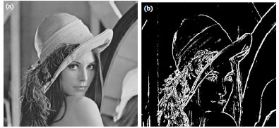 | |
| Fig. 6(a-b): | Edge-detection output images |
| Table 2: | Comparison of architectures |
 | |
| *Includes only ports for pixels and output MV, FLP: Frame level pipelining | |
| Table 3: | Device Utilization Statistics with target device xc4vsx25-12ff668 |
 | |
| *Including control pins | |
Figure 6 shows the edge-detected image of Lena. The device utilization for both the modules is shown in the Table 3.
CONCLUSION
A new heuristic for reducing the search space based on the dependence vectors was presented in this paper. A four level nested loop representation for FSBM algorithm was also shown. Based on this approach FSBM and ED algorithms were implemented for image size of 256x256 pixels and 512x512 pixels, respectively. Further the PEs of ED and FSBM architectures can be combined to realize a reconfigurable image processing hardware.
REFERENCES
- Lee, P. and Z.M. Kedem, 1988. Synthesizing linear array algorithms from nested for loop algorithms. IEEE Trans. Comput., 37: 1578-1598.
CrossRef - Komarek, T. and P. Pirsch, 1989. Array architectures for block matching algorithms. IEEE Trans. Circuit Syst., 36: 1301-1308.
CrossRef - Kumar, V.K.P. and Y.C. Tsai, 1991. On synthesizing optimal family of linear systolic arrays for matrix multiplication. IEEE Trans. Comput., 40: 770-774.
CrossRef - Kittitornkun, S. and Y.H. Hu, 2001. Frame-level pipelined motion estimation array processor. IEEE Trans. Circuits Syst. Video Technol., 11: 248-251.
CrossRef - Kittitornkun, S. and Y.H. Hu, 2003. Mapping deep nested do-loop DSP algorithms to large scale FPGA array structures. IEEE Trans. Very Large Scale Integr. Syst., 11: 208-217.
CrossRef - Yeo, H. and Y.H. Hu, 1995. A novel modular systolic array architecture for full-search block matching motion estimation. IEEE Trans. Circuit Syst. Video Technol., 5: 407-416.
CrossRef