
B. Jothi Mohan
Department of ECE, Anna University, Chennai 600 025, India
V.C. Ravichandran
Department of ECE, Anna University, Chennai 600 025, India
Information Technology Journal
Year: 2007 | Volume: 6 | Issue: 2 | Page No.: 283-287


ABSTRACT
In this study resource allocation in ad hoc network is formulated, as a utility maximization problem the constraint considered is rate constraint. Rate constraint is defined such that the traffic flow from source node to the destination should be less than the net channel capacity between them but at the optimum value. In cross layer design optimization of rate constraint can be done using three layer constraints namely congestion constraint of transport layer, routing constraint of network layer, schedulable constraint of link layer. These three components form the core components of rate optimization. We formulate a congestion price to interact with congestion constraint, routing constraint and scheduling constraint in a fixed wireless channels. This principle can be extended to time varying channel and multi-rate devices. Here in this study we establish a relationship between congestion window and local congestion price. Resource allocation namely wireless links of fixed bandwidth is done to optimize these constraints. We are considering this problem as utility maximization with the constraints of rate, routing and scheduling. The resources considered are inter nodal paths of fixed channel bandwidths, for optimal utilization. Let us look at the resource allocation problem using congestion price as the flow variable. We prove the convergence of the algorithm. In this analysis we have considered time invariable and fixed rate devices. The stability of the system is established. Its performance is characterized with respect to an ideal reference system which has the optimum rate region at link layer. The congestion window is adjusted by values of local source rate constraint.
PDF Abstract XML References Citation
How to cite this article
B. Jothi Mohan and V.C. Ravichandran, 2007. Cross Layer Optimization for Congestion Control in Adhoc Networks. Information Technology Journal, 6: 283-287.
DOI: 10.3923/itj.2007.283.287
URL: https://scialert.net/abstract/?doi=itj.2007.283.287
DOI: 10.3923/itj.2007.283.287
URL: https://scialert.net/abstract/?doi=itj.2007.283.287
INTRODUCTION
The seven layer Open System Integration (OSI) architecture offers simplicity and modularity but optimizing within layers has reached the point of diminishing returns. Future applications that will fuel the growth of wireless demands orders of magnitude in performance improvement. The Cross-layer Dilemma is efficiency vs. modularity but Cross-Layer design is needed to improve efficiency. OSI Layers are modular. Loss of modularity in cross layer design is possible (Kumar and Gupta, 2001). Hence overall cross-layer solution must ensure both efficiency and modularity. It is believed by the authors an appropriately designed cross-layer solutions should exhibit a layered structure with minimal but crucial interaction between the layers.
To determine the maximum end-to-end rate at which users should transmit and at the same time find the associated scheduling policy that stabilizes the system is a cross-layer problem. The power levels determine the performance of medium access control in the link layer based on the contention for the medium depends on the number of nodes within the range of reference.
Traditionally, network protocols take a strictly layered structure and implement congestion control, routing and scheduling independently at different layers. However, wireless spectrum is a very scarce resource and it is important to use the wireless channel efficiently. In order to achieve high end-to-end throughput and efficient resource utilization, congestion control, routing and scheduling should be jointly designed while the architectural separation among them is preserved.
The need for joint design across these three layers is motivated by three observations. First, wireless channel is a shared medium and interference-limited unlike in wire line networks where links are disjoint resources with fixed capacities. In adhoc wireless networks the link capacities can be construed as elastic and the contention among links provide a fundamental constraint for resource allocation (Chen et al., 2005). They determine the feasible rate region at link layer. Second, most routing schemes for ad hoc networks select paths that have minimum hop counts (Johnson et al., 2005; Perkins et al., 1999). This implicitly predefines a route for any source-destination pair of a static network, independent of the pattern of traffic demand, interference or contention among links. This may result in congestion at some region while other regions are under-utilized. To use the wireless spectrum more efficiently, we should exploit multiple paths based on the pattern of traffic demand, interference and contention among links. As routing is then determined from the rate and scheduling constraints. Lastly, TCP congestion control algorithms can be interpreted as distributed primal-dual algorithms over the Internet to maximize aggregate utility, (Kelly et al., 1998; Low and Lapsley, 1999; Kunniyur and Srikant, 2003). This series of work implicitly assumes a network where link capacities are fixed and routes are pre-specified. Here, we extend the basic utility maximization formulation with rate constraints at source nodes and additional constraints on scheduling at link layer.
Shannon has shown the channel capacity C is given by
C = log2(1+Es/Ns) |
Where Es/Ns is the signal to noise ratio.
MODEL DETAILS
We consider an ad hoc wireless network with a set of N nodes and a set of L logical links of finite capacity of Cl Bits sec-1. These links are directed and we assume connectivity to be symmetric meaning,
l(i,j)ε {L} if and only if l(j,i) ε {L} |
We assume a static topology meaning the nodes are immobile and each link l has a fixed finite capacity cl bits per second. i.e., we implicitly restrict that the wireless channel is a fixed one or by some underlying mechanism it is achieved, so that the wireless channel appears to have a fixed rate. But, wireless channel is a shared medium and interference-limited where links contend with each other for exclusive access to the channel hence we have to relax this restriction. We will build a conflict graph to capture the contention relationships among the links. Independent set of links are the ones which do not have common node. Thus the maximum feasible rate region at link layer is the convex hull of the corresponding rate vectors of independent sets of this conflict graph. We will introduce another multi-commodity flow variable, which correspond to the link capacities allocated to the flows towards different destinations, to describe the rate constraint at network layer. The resource allocation is then formulated as a utility maximization problem with schedulable and rate constraints described.
Schedulable constraints and rate constraints: As discussed we consider a network with primarily interference links. A node that share a common link cannot transmit or receive simultaneously. Links that do not share nodes can transmit and receive and are called independent nodes.
 | |
| Fig. 1: | An ad hoc wireless network 4 nodes in chain topology (A,B,C,D) 6 logical links (1, 2, 3, 4, 5, 6) |
 | |
| Fig. 2: | The conflict graph |
The same interference model has been used in (Kodialam and Nandagopal, 2003, Xiao et al., 2005). This models a wireless network with multiple channels available for transmission. For example, simultaneous communications in a 802.11 compatible Network Interface Cards (NIC) has 12 channels. Under this defined interference model, we can construct a conflict graph (Jain et al., 2003; Low, 2003) that captures the contention relationship among the links. In the conflict graph, each vertex represents a link and an edge between two vertices denotes the contention between the two corresponding links. These links cannot transmit at the same time. Figure 1 shows an example of a wireless ad hoc network and its conflict graph (Fig. 2).
Network model: The model considered here is a set of 4 nodes. The links are 1, 2, 3, 4, 5, 6 are symmetric.
The independent sets of vertices in the conflict graph are the ones which do not have common edges. Eg: {1,5} or in general terms {e}. An independent set e as a |L|-dimensional rate vector re.. where the lst entry is
rel.: = cl capacity of the lth link if lε e else 0 |
The feasible region in the link layer is defined as the convex hull of these rate vectors re represented as Ř.
 |
If y is the link flow vector then according to schedulablity constraint it should belong to the region Ř
Se is the transmission schedule of the network at an instant of time. Transmission schedule of each source node during a period of time is fixed by this constraint.
Let D denote the set of destination nodes of network layer flows.
Let fki,j be the allocated capacity flow to destination k.
Let xki,j be the flow generated from I to k through j. and
This flow should not exceed the summation of the capacities of incoming and outgoing flows Symbolically
(2) |
where I,ε N and kε D j ≠ k.
This equation is the rate constraint for resource allocation We interpret the multi-commodity flow variable as the flows of different destinations. The amount of link capacities allocated in the network during that schedule to different destinations is taken as the multi commodity flow variable.
PROBLEM FORMULATIONS
We use l ε L to denote a link. We assume there is at most one flow between any node and destination pair (i,k). (This restriction can be relaxed by induction).
Let s to denote a network layer flow between the source destination pairs (I,k).
We define a utility function U as continuously differentiable, Increasing and strictly concave.
Let Us(Xs) denote the utility attained by a source s at a source rate of Xs.
(3) |
(4) |
the flow fεŘ | (5) |
Where Iε N kε D I ≠ k | (6) |
Solving the system problem (4)-(5) directly,
Our problem is to choose source rates xs with allocated capacities fki,j so as to solve the global problem of rate maximization Equation (3) states the net utility of the flow x from I to k via j which is the one to be maximized.
Equation (4) states the flow x should be less than or equal to the net channel capacities allocated.
Equation (5) states the flow x should belong to the region of flow.
To solve these system problems directly we need the coordination among possibly all sources and links in the network. Since (3) is a convex optimization problem with strong duality distributed algorithms can be used. Hence form the Lagrange dual problem and interpret the resulting algorithm in the context of joint design of congestion control, routing and scheduling.
Dual decomposition for cross-layer design
Formulation of dual algorithm: Let D(p) be the Dual to the problem of the equation (3) with the constraints of (4) and (5) then
 |
By this we introduce the Lagarange multiplier Pki for the source I and destination k.
Now Eq. (7) can be decomposed into two problems
(8) |
(9) |
We can interpret pki as the congestion price the first sub problem is congestion control (Low and Lapsley, 1999; Asmussen, 2003) and the second is the rerouting and scheduling Thus the flow global optimization problem decomposes into separate local optimization problem of transport and network/link layer with congestion price as the interaction parameters.
Congestion control
Consider the Eq. (8)
when LHS D1(p) tends to zero (min)
xs(p) = U t-1s(ps) | (10) |
Equation (10) adjusts the source rate according to the congestion price of the source node, this is different from TCP which uses the aggregate price along its path.
We can also rewrite it as
(11) |
Price adjustment for a pair of source destination pair (I,k) is given by
pki(t+1) = [pki(t)+Υt(xki (p(t))- (-(Σ fki,j (p(t))- Σfkj,I (P(t)))] | (12) |
where Υt is a positive scalar step size which is the most important parameter
Operation of the algorithm: If the demand xki (p(t)) for bandwidth at source node I for a flow to destination exceeds the effective capacity Σ fki,j - Σ fkj,I, then the price pki will raise which in turn will reduce the demand and increases the effective capacity Thus the dual algorithm motivates a joint congestion control, routing and scheduling design wherein at the transport layer sources s individually adjust their rates according to the local congestion price and also nodes I individually updates their prices according to Eq. (11) and at the network/link layer nodes I solve the scheduling and route work/link layer data flows accordingly.
NUMERICAL MODEL
Figure 3 shows a network of 6 nodes named A,BC.D,E,F. A and B form members of source set and E is the destination.
Two network layer flows are considered A to F and B to E with the utility function of
Us(xs) = log(xs) |
All the channels are of fixed capacity. This can be relaxed as elastic channel. So, the devices at the nodes are of fixed rate devices. So the links considered are of fixed capacity. The symmetric links {(C,E),(E,C)} and {(B,F),(F,B)} are of capacity 1 unit and all others are considered to have 2 units.
Two Algorithms are simulated for I) Perfect scheduling ii) distributed scheduling.
Perfect scheduling: We evaluate source rate and congestion price of each flow the step size is Υ = 0.1
Figure 4 shows that they converge to a neighborhood of the optimal and then oscillate around the optimal This oscillations can be construed as non differentiability of the dual function and physically due to the scheduling process.
However, Fig. 5 shows the average source rates and congestion price are smooth approaches the optimum monotonically.
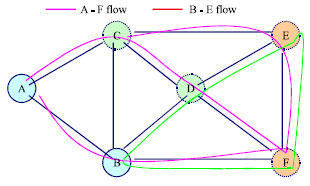 | |
| Fig. 3: | A network with simultaneous network layer flows |
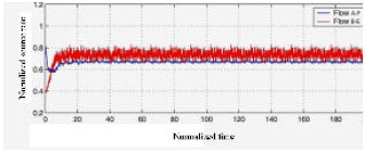 | |
| Fig. 4: | Source rate and congestion price with perfect scheduling. X axis normalized source rate; Y axis normalized time |
 | |
| Fig. 5: | Source rate and congestion price with perfect scheduling. X axis normalize congestion rate.; Y axis normalized time |
The performance of the algorithm is better than the average bound of ΥG2/2. Table 1 and 2 shows the average link rates allocated to each flow between the source and destination in a perfect schedule scheme.
Distributed scheduling: The evolution of source rates, congestion prices and there are similar to those with perfect scheduling they converge quickly to a neighborhood of stable values (Fig. 6). The source rates are less than those achieved with perfect scheduling since the feasible rate region hub is smaller under the distributed scheduling (approximate scheduling.) Table 3 and 4 summarizes the average link rates allocated to each flow. But we notice the routing pattern change. Every link is used in routing unlike in the previous case B to C was not used in this case the links can be locally heaviest link.
 | |
| Fig. 6: | Source rate and congestion price with distributed Scheduling. X axis normalized congestion rate. Y axis normalized time |
| Table 1: | Average flow rates A to F in units Individual link flows shown |
 | |
| Table 2: | Average flow rates B to E in units |
 | |
| (Perfect scheduling) | |
| Table 3: | Average flow rates A to F in units individual link flows shown |
 | |
| Table 4: | Average flow rates B to E in units |
 | |
| (Distributed scheduling) | |
The worst case performance bound is ½ the simulation results show that the degradation of the performance of Perfect schedule algorithm is small. This schedule has very low communication overhead, very fast convergence and good performance this design is promising for practical implementation.
CONCLUSIONS
This model is for the joint design of congestion control routing and scheduling for wireless ad hoc networks the frame work network utility maximization is used with the application of dual-based decompositions. We have formulated two algorithms for with fixed wireless channels (single-rate wireless devices) as a utility maximization problem for overall system’s degradation due to suboptimal design in one layer. We have proved the rate optimization for fixed channel model this can be extended to elastic models.
REFERENCES
- Gupta, P. and P.R. Kumar, 2000. The capacity of wireless networks. IEEE Trans. Inform. Theory, 46: 388-404.
CrossRefDirect Link - Kunniyur, S. and R. Srikant, 2003. End-to-end congestion control schemes: Utility functions, Random losses and ECN marks. IEEE/ACM Trans. Network., 11: 689-702.
CrossRef - Low, S.H., 2003. A duality model of TCP and queue management algorithms. IEEE/ACM Trans. Network., 11: 525-536.
CrossRef - Perkins, C.E. and E.M. Royer, 1999. Ad-hoc on-demand distance vector routing. Proceedings of the 2nd Workshop on Mobile Computing Systems and Applications, February 25-26, 1999, New Orleans, LA., pp: 90-100.
CrossRef