
N. Yusoff
Department of Chemical Engineering, Universiti Teknologi PETRONAS, Bandar Seri Iskandar, 31750 Tronoh, Perak, Malaysia
M. Ramasamy
Department of Chemical Engineering, Universiti Teknologi PETRONAS, Bandar Seri Iskandar, 31750 Tronoh, Perak, Malaysia
Journal of Applied Sciences
Year: 2010 | Volume: 10 | Issue: 24 | Page No.: 3313-3318


ABSTRACT
This study presents a procedure for selecting optimization variables in a Refrigerated Gas Plant (RGP) using Taguchi method with L27 (39) orthogonal arrays. A dynamic RGP model developed under HYSYS environment is utilized as a test bed. This model comprises 762 variables and 21 regulatory control loops. However, only 9 variables or factors with three level each are studied to determine their relative significance in maximizing RGP profit. These factors are prudently selected due to their relevance in maintaining product qualities. Feed Gas (FG) flow rate is found dominant with 97.3% contribution in the first case study. Two additional case studies are performed to magnify the contributions of other factors. FG costs and temperature of FG after coldbox E-101, refrigeration cooler duty and demethanizer reboiler duty are found to be significant factors.
PDF Abstract XML References Citation
Received: June 06, 2010;
Accepted: July 06, 2010;
Published: October 19, 2010
How to cite this article
N. Yusoff and M. Ramasamy, 2010. Selection of RGP Optimization Variables using Taguchi Method. Journal of Applied Sciences, 10: 3313-3318.
DOI: 10.3923/jas.2010.3313.3318
URL: https://scialert.net/abstract/?doi=jas.2010.3313.3318
DOI: 10.3923/jas.2010.3313.3318
URL: https://scialert.net/abstract/?doi=jas.2010.3313.3318
INTRODUCTION
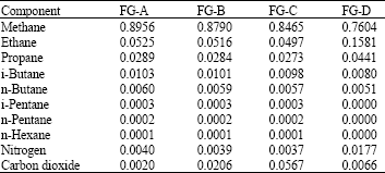
A Refrigerated Gas Plant (RGP) processes raw Feed Gas (FG) into Sales Gas (SG) and Natural Gas Liquids (NGLs). Among challenges faced by an RGP operator are fluctuations of FG flow rates and compositions as well as different contractual terms at both inlets and outlets. Operating RGP at optimum conditions can improve its profit margin. Since hundreds of variables are available for manipulation, proper selections of optimization variables, or factors, are required. These factors need to be evaluated using a test bed. A dynamic model of RGP developed under HYSYS environment by Yusoff (2009) is suitable for this purpose (Fig. 1). This large model contains 762 variables and 21 regulatory control loops. Feeds to RGP come from three main streams FG-A, FG-B and FG-C. Another feed stream (FG-D) is available in smaller quantity to boost SG Gross Heating Value (GHV). The feed gas compositions vary as listed in Table 1.
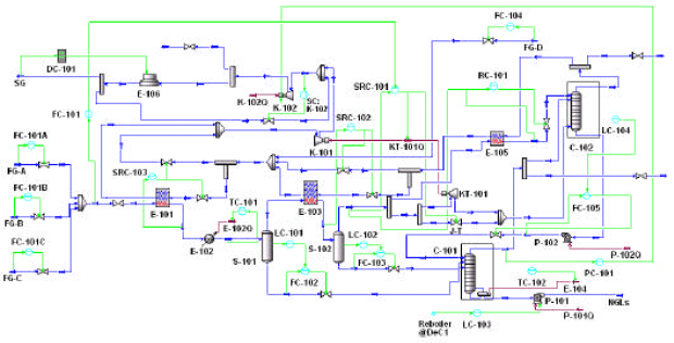 | |
| Fig. 1: | RGP process flow diagram |
| Table 1: | Feed gas compositions |
 | |
In this study, Taguchi method for design of experiment (DOE) and analysis of variance (ANOVA) is applied: (1) to quantify relative importance of 9 factors, (2) to determine optimum configurations of factors and (3) to estimate and validate optimum output (Roy, 1990). Taguchi method has been successfully applied in many engineering disciplines. Cheng et al. (2008) studied thermal chemical vapor decomposition of silicon by integrating computational fluid dynamic codes in FLUENT and a dynamic model of Taguchi method with L18 (21x37) OAs. Engin et al. (2008) investigated color removal from textile dyebath effluents in a zeolite fixed-bed reactor employed L16 (42x22) OAs. Chiang (2005) presented an effective method for predicting and optimizing cooling performance of parallel-plain fin heat sink module using L18 (21x37) OAs. Lee and Kim (2000) proposed a new controller gain tuning technique based on L9 (34) OAs with application in a simultaneous multi-axis PID control system.
In the current research, L27 (39) OAs are utilized since there are 9 factors at 3 level each. Three case studies are performed to defuse dominance of plant load and FG costs in determining RGP profit. Case 1 involves all 9 factors. In Case 2, plant load is removed from Taguchi orthogonal arrays (Taguchi et al., 2000). RGP load is maintained at 250 t h-1. In Case 3, both plant load and FG costs are removed whereas other factors are shifted down by a row to ensure unbiasedness of experimental design. Similar to Case 2, plant load is kept at 250 t h-1. However, only FG-A is processed by RGP.
An objective function below is applied to determine the performance of individual factors.
| (1) |
where, profit P is the difference between revenues Ri and expenses Ej of all contributors i=1,…,I (I=5) and j=1,…, J (J=10), respectively. In this study, revenues come from the values of SG and NGLs comprising ethane, propane, butane and condensates.
| Table 2: | Economics data |
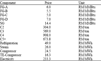 | |
| Source: Personal correspondence with an engineer working at a GPP | |
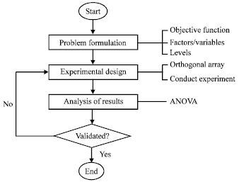 | |
| Fig. 2: | Flow diagram of Taguchi method |
Expenses are mainly due to costs of feed gases (FG-A to FG-D) and utilities in the forms of E-102 cooler duty, C-101 reboiler duty, compressor fuel gas consumption, turboexpander-compressor maintenance and electricity usage for pumping actions. Prices and corresponding units of each component of revenues and expenses are shown in Table 2.
TAGUCHI METHOD
Taguchi method can be illustrated as a flow diagram in Fig. 2. The procedure employed in the current work is modified from that presented in reference (Yang et al., 2007). It is more compact and includes a failure loop for invalidated DOE. Step 1 is problem formulation, which requires defining an objective function, factors and levels. This step requires an in-depth knowledge of the process of interest. In case of RGP, inputs from experienced operators are essential in determining potential optimization variables, as well as their normal, high and low values (Table 3). Variables are called factors or parameters in Taguchi-related literature. Limits of high and low values are called levels.
| Table 3: | Description of factors, variables and levels |
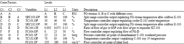 | |
Median and lower and upper quartiles of the limits may also be included to augment experimental design configurations.
Step 2 involves designing and conducting experiments. Numbers of factors and levels have an effect on selection of standard orthogonal arrays. For 9 factors and 3 levels such as the one in this study, an L27 array consisting of 27 rows and 13 columns is selected. The rows and columns represent experimental runs and factors, respectively. Since, only 9 factors are used to calculate RGP profit, the remaining 4 columns on far right of the array are ignored. It is noted that, in order to capture adequate responses of all 9 factors towards the objective function, only 27 experiments need to be run for one case study under Taguchi method. This is more appealing than running 19,683 (39) experiments under full factorial design approach.
Step 3 deals with analysis of results. A statistical tool commonly applied is analysis of variance (ANOVA). Two averages are calculated a priori before performing ANOVA. Average of factor k over level l, ![]() is taken as sum of all factors divided by number of repeated level, NR.
is taken as sum of all factors divided by number of repeated level, NR.
| (2) |
Another one is average of factor k over all levels L, ![]() as defined below:
as defined below:
| (3) |
These two averages are used to calculate variance Vk, which has two contributors. The numerator is sum of squares between two averages of factor ![]() . The denominator is called degrees of freedom of factor k over all levels L (DOF)k.
. The denominator is called degrees of freedom of factor k over all levels L (DOF)k.
 | (4) |
Percentage contribution Ck is obtained by dividing individual variance of factor k, Vk from total variance of all factors and multiplying the result with 100.
 | (5) |
Step 4 is validation of experiment. For each case in this study, there are 27 combinations of experimental runs. By design, only one will yield the highest profit margin. Preliminary visual inspection of trends of each factor average contributions at all levels is possible through an effect plot. Here, average values of factor k, ![]() are plotted against all levels l=1,…,L (L =3). The effect plot may be used to locate optimum design configuration for the purpose of verifying results. This means that an additional experiment is run to compare both experimental and calculated outputs (profit). The calculated optimum profit xopt is obtained by summing up global mean
are plotted against all levels l=1,…,L (L =3). The effect plot may be used to locate optimum design configuration for the purpose of verifying results. This means that an additional experiment is run to compare both experimental and calculated outputs (profit). The calculated optimum profit xopt is obtained by summing up global mean ![]() with maximum deviations of average of factor k over all levels l=1,…,L,
with maximum deviations of average of factor k over all levels l=1,…,L, ![]() from its corresponding average
from its corresponding average ![]() .
.
| (6) |
where
| (7) |
Equation 7 implies that average of factor k, ![]() over all levels equals to global mean
over all levels equals to global mean ![]() . This is true since Taguchi OA is unbiased by construction.
. This is true since Taguchi OA is unbiased by construction.
RESULTS AND DISCUSSION
All experiments are conducted in RGP dynamic model developed under HYSYS environment. Profit (Eq. 1) is calculated online in a built-in spreadsheet. Material and energy units are converted a priori to be consistent with the basis of 1 min interval calculation.
| Table 4: | Results of anova for case 1 |
 | |
| Table 5: | Results of ANOVA for case 2 |
 | |
| Table 6: | Results of ANOVA for case 3 |
 | |
To ensure repeatability, HYSYS 2006 SP5 running on Windows XP Professional system is employed. Reproducibility is also ensured because experimental steps are pre-configured in Event Scheduler. Changes on levels of all factors are set to run in parallel. Experiments are stopped after all factors reach steady-state at 420 min (7 h) simulation time. In most experiments, profit values level off after 360 min but in some runs, the values slightly fluctuate towards the end. For these runs, the last 60 values are averaged out. Therefore, only one profit value is required for each run.
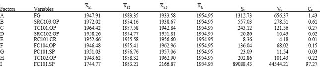
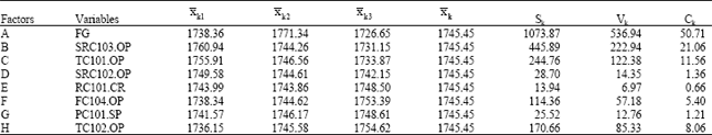
To study relative significance of factors quantitatively, ranking of factors is performed using ANOVA. Tables 4, 5 and 6 show ANOVA results for Cases 1, 2 and 3. Initially, Eq. 2 and 3 are applied to calculate averages of factor k. These two averages are used to determined sum of squares of factor k, Sk. In general, Sk values represent deviation of experimental results of factor I from data average. A large value such as the one obtained here indicates significant contribution of that particular factor towards output (RGP profit).
On the other hand, a factor is deemed unimportant if its Sk value approaches zero. Since, Sk values are unbounded at the higher end, it is convenient to denote relative importance of a factor k in term of its percentage contribution, Ck. The Ck values of all factors in Cases 1, 2 and 3 are calculated from Eq. 5. Before calculating Ck, a quantity called general variance of factor k, Vk needs to be determined. This quantity differs from population variance σ2, which could only have been obtained if all 19,683 (39) possible experiments are conducted. Vk is obtained from Eq. 4 where degree of freedom of factor k, (DOF)k is one less its number of levels. Other Ck values for Case 1 are calculated using the same procedure and presented in Table 4.
The descending order of importance of all 9 factors is IABCHFGDE. It is clear that factor I (plant load) with contribution of 97.3% is too dominant. Increasing plant load increases amount of FG and thus RGP profit due to additional productions of SG and NGLs. However, it should be noted that RGP was designed to process a maximum of 310 t h-1 of FG. Any amount higher than this will push equipment loads towards upper constraints. On the other hand, RGP load can be reduced to 100 t h-1 of FG without the need for total plant shutdown. However, under-loading is undesirable since RGP profit will also diminish. Total contribution from other factors in Case 1 is only 2.7%. To magnify relative significance of these factors, two more case studies are conducted.
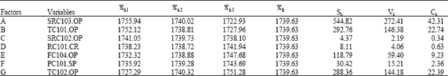
Case 2 deals with a study on effects of factors A to H on RGP profit. The descending order of importance of all 8 factors is ABCHFDGE (Table 5). Factor A (FG streams) is the most significant factor with 50.7% contribution. This is attributed to different economic values of FG streams A, B and C due to varying levels of carbon dioxide contents (Table 1). Highly priced FG-A erodes RGP profit while cheaper FG-C increases it. About one-third contribution to RGP profit comes from factors B (SRC103 output) and C (TC101 output). These two factors essentially control RGP temperature. Increasing values of factors B and C decreases RGP temperature and thus increases NGLs recovery. Adjustment of factors B and C affects separation of SG from NGLs at demethanizer column (C-101).
Consequently, reboiler duty (factor H or TC102 output) needs to be adjusted as well. Contribution of factor H in Case 2 is about 8%. Another 5.4% contribution comes from factor F (FC104 output), which regulates re-injection of rich hydrocarbon to boost SG gross heating value. However, it should be noted that only 10 ton h-1 of FG-D is available for this purpose. The remaining FG-D, which is produced by a neighboring plant, is reserved for an existing customer. Minor contributions of about 1% come from factors D (SRC102 output) and G (C-101 overhead pressure). Both factors are mainly used to regulate C-101 overhead quality. Since installation of Gas Subcooled Process (GSP) section in RGP, the influence of factors D and G on C-101 overhead quality have been significantly reduced. The smallest contribution of 0.7% comes from factor E (RC101 ratio). This factor regulates split of processed gas going into GSP and/or turbo-expander. A higher value of factor E promotes more recovery of ethane and heavier components at GSP.
The effect of 7 factors is examined in Case 3 where only FG-A is fed to RGP. In other words, FG stream factor is removed from Taguchi array and replaced with SRC103 output. Factor A is now SRC103 output, which was previously factor B in Cases 1 and 2. Other factors are also moved down one place to complete the array as shown in Table 3. The moves are necessary to uphold unbiasedness of Taguchi method. The descending order of importance is ABGEFDC (Table 6).
As revealed from Case 3 results, SRC103 output is a major contributor with 42.3%. This factor regulates temperature of FG exiting coldbox E-101 that could influence refrigeration cooler duty (TC101 output). Lower FG temperature mean less cooler duty is required to maintain same separation and thus higher RGP profit. Under this circumstance, contributions coming from TC101 output and TC102 output are equivalent at about 22%. An increase in TC101 output further reduces RGP temperature. To maintain RGP overall energy balance, TC102 output should be raised accordingly. The effect of FC104 output in Case 3 is more significant with 9.2% contribution. An increase in FC104 output, thus hydrocarbon re-injection through FG-D, increases SG production.
Due to large disparity of SG and FG-D prices (Table 2), a lift in SG rate increases RGP profit. For Case 3, contribution of PC101 output is almost seven times as large as SRC102 output. This implies that PC101 output is more effective than SRC102 output in regulating C-101 overhead quality. This condition is most likely due to leaner composition of hydrocarbon in FG-A, which causes separation of SG from NGLs in C-101 to be dominated by pressure-swing rather than temperature-swing action. The contribution of RC101 ratio remains minor in Case 3. This factor is useful in improving ethane recovery in GSP but less significant in increasing RGP profit.
The final step in Taguchi method is validation of results. Here, RGP profits obtained from running experiments in HYSYS are compared with those calculated based on ANOVA results. For Cases 1, 2 and 3, optimum levels of factors are determined from the maximum values of factorial average (Table 4-6). In Case 1, it is clear that the highest RGP profit could be obtained from configuration A2B1C1D3E3F3G3H3I3. This optimum configuration is set in HYSYS Event Scheduler and run for 420 min to yield RGP profit of 2241.18. This value is compared with 2244.85, which is obtained from Eq. 6. Comparing outputs obtained from HYSYS experiment and ANOVA table, a small deviation of 0.16% entails that an optimum configuration is found. The same procedure is applied for other two cases. In Case 2, configuration A2B1C1D1E3F3G3H3 (K=8) produces optimum outputs of 1823.80 (HYSYS) and 1824.75 (ANOVA) with 0.05% deviation. In Case 3, RGP profits of 1798.38 (HYSYS) and 1795.92 (ANOVA) with 0.14% deviation are obtained from configuration A1B1C1D3E3F3G3 (K=7). Since deviations of outputs obtained at optimum factor configurations are small, the final objective of this study is achieved.
CONCLUSION
Three case studies were performed to determine relative importance of 9 factors based on ANOVA. In Case 1, FG flow rate was found to be the most dominant factor at 97.3%. To magnify contributions from other factors, two more case studies were conducted. Cases 2 and 3 involve 8 and 7 factors, respectively. FG costs with about one-half contribution were a significant factor in Case 2. When this factor was removed in Case 3, a significant contribution of 42.3% came from SRC103 output, which regulates FG temperature by splitting SG flow to coldbox E-101. In addition, contributions from external cooling and heating factors were found to be equivalent.
Maximum RGP profit was derived from an optimum configuration of factors. This unique configuration of low, medium or high levels of individual factors was selected based on an effect plot and set in HYSYS for validation. In each case study, results from HYSYS experiments were compared against those from ANOVA table. Remarkable agreements found in all case studies show that an optimum configuration of factors would yield maximum RGP profit.
ACKNOWLEDGMENT
The authors express gratitude to Universiti Teknologi PETRONAS (UTP) for providing financial assistance.
NOMENCLATURE
| Ck | : | Percentage contribution of factor k |
| E | : | Expenses |
| L | : | No. of levels |
| P | : | Profit |
| R | : | Revenues |
| Vk | : | Variance of factor k |
| : | Average of profit | |
| : | Average of profit due to factor k over all levels L | |
| : | Average of profit due to factor k at level l | |
| : | Optimal profit |
Abbreviation
| ANOVA | : | Analysis of variance |
| DOE | : | Design of experiment |
| DOF | : | Degrees of freedom |
| FG | : | Feed gas |
| NGLs | : | Natural gas liquids |
| OA | : | Orthogonal array |
| RGP | : | Refrigerated gas plant |
| SG | : | Sales gas |
REFERENCES
- Cheng, W.T., H.C. Li and C.N. Huang, 2008. Simulation and optimization of silicon thermal CVD through CFD integrating Taguchi method. Chem. Eng. J., 137: 603-613.
CrossRef - Engin, A.B., O. Ozdemir, M. Turan and A.Z. Turan, 2008. Color removal from textile dyebath effluents in a zeolite fixed bed reactor: Determination of optimum process conditions using Taguchi method. J. Hazard. Mater., 159: 348-353.
CrossRef - Chiang, K.T., 2005. Optimization of the design parameters of parallel-plain fin heat sink module cooling phenomenon based on the Taguchi method. Int. Commun. Heat Mass Transfer, 32: 1193-1201.
CrossRef - Lee, K. and J. Kim, 2000. Controller gain tuning of a simultaneous multi-axis PID control system using the Taguchi method. Control Eng. Prac., 8: 949-958.
CrossRef - Yang, K., E.C. Teo and F.K. Fuss, 2007. Application of taguchi method in optimization of cervical ring cage. J. Biomech., 40: 3251-3256.
Direct Link