
Juan C. Matallin-Saez
Departamento de Finanzas y Contabilidad, Universitat Jaume I, 12070, Castellon, Spain
Journal of Applied Sciences
Year: 2009 | Volume: 9 | Issue: 9 | Page No.: 1776-1780


ABSTRACT
The objective and contribution of this study is to analyse market timing over non-simultaneous periods. This approach considers that decisions on portfolio risk could affect the fund return in subsequent periods and not only the simultaneous period. Robust estimates of changes in beta are computed by Kalman filtering. Initial results for a sample of Spanish mutual funds do not evidence market timing ability in general, although a higher number of funds, particularly larger funds, present negative timing. The study shows how the evidence of negative timing is more robust and persistent for a longer term window. For shorter terms the evidence is driven by an omitted benchmark bias from negative timing of small cap stocks. A comparison of these results with those achieved by a set of passive benchmarks following a buy and hold strategy demonstrates that the long term evidence of negative timing in mutual funds is the result of management contrary to a buy-and-hold strategy.
PDF Abstract XML References Citation
How to cite this article
Juan C. Matallin-Saez, 2009. Non-Simultaneous Market Timing in Mutual Funds. Journal of Applied Sciences, 9: 1776-1780.
DOI: 10.3923/jas.2009.1776.1780
URL: https://scialert.net/abstract/?doi=jas.2009.1776.1780
DOI: 10.3923/jas.2009.1776.1780
URL: https://scialert.net/abstract/?doi=jas.2009.1776.1780
INTRODUCTION
The financial literature on mutual fund performance has developed significantly alongside the growth of the funds industry. One stream of research in this literature concerns the market timing ability of mutual funds. Correct (perverse) timing implies that managers increase (decrease) fund risk to anticipate an upward (downward) stock market. When evaluation of market timing is based on returns data, a model is generally introduced that explains how the fund returns are generated and how the timing decisions are incorporated. The most widely used models in the literature involve a linear relation between the fund returns and the market. Taking the linear model as a base, the most common procedure in the literature is to introduce a quadratic term to measure market timing (Holmes and Faff, 2004). Thus, the beta of the fund is equal to a constant and a slope with respect to market return. Correct (perverse) timing implies an increase (decrease) in the beta in an upward (downward) market. On the other hand, Henriksson and Merton (1981) propose a model with two levels of beta, for up and down markets, respectively. A large number of empirical studies have applied these models and others derived from them, to measure market timing. These studies, from Henriksson and Merton (1981) to Holmes and Faff (2004), do not find evidence of timing in general, but in some cases find perverse timing. Ferson and Schadt (1996) also used returns although with a different methodology; in general they find no evidence of timing, but in some cases positive timing was found. These researchers propose a conditional approach that allows a variable beta over time according to managers’ response to public market information. Matallín (2008) also proposes a time varying beta to evaluate portfolio timing. These studies show how a beta that is not constant over time can provoke artificial timing. To avoid this, market timing should be evaluated over short periods. Benos and Jochec (2008) use daily return data to look for persistence in the ability of mutual funds to time the market, finding persistence only among well performing funds.
In general, earlier evaluations of market timing ability have proposed models, with either a constant or time-varying beta, that consider simultaneous timing. That is, these models compare the beta in a period with the market return in the same period. However, the portfolio management in a period could be a forecast of market movements in upcoming periods. For example, consider a manager that times an upward market in the next period and increases the beta of the portfolio at the beginning of the t day. The situation may occur in which the market does not rise on this day, but it rises sharply on following days. If simultaneous days are compared, the evidence will be of no timing, although timing has taken place. This problem could be solved by measuring timing over wide periods. However, Goetzmann et al. (2000) and Bollen and Busse (2001) showed how the evaluation of short term timing could be biased when it is measured over wide periods. The present study aims to solve non-simultaneous timing by measuring it over windows of varying length ranges.
DATA AND MUTUAL FUND SAMPLE
In the empirical section of the study, a sample of Spanish mutual funds (FIM, Fondos de Inversión Mobiliaria) is analysed. Mutual fund daily net share values, from July 1998 to September 2004, were provided by the Spanish Stock Market National Commission (CNMV). The sample was made up of all the risky mutual funds in the period sample, specifically 79 mutual funds that mainly invest in equities in the domestic stock market. The IGBM, the Madrid Stock Exchange Index, was used as a proxy for the Spanish stock market. This value-weighted index was chosen because it holds a large number of equities and may better represent the diversified portfolios of the sample mutual funds. The return implicit in T-bills repos is used as risk-free return. The data sources used were Internet information providers from the Madrid Stock Exchange and the Analistas Financieros Internacionales (AFI).
In addition, the effect of omitted benchmarks when evaluating market timing is also considered. To do this, an additional, equally-weighted benchmark is constructed with medium and small cap stocks, (EMS benchmark). Harvey and Siddique (2000) and Barone-Adesi et al. (2004) have shown how small stocks present negative coskewness with respect to the market. If this is not controlled for, even in a passive portfolio without timing management, artificial evidence of negative timing may be found because the assets held by the fund show this behaviour. Daily returns from stock prices data, provided by Intertell, are used to construct the EMS benchmark.
This study presents the results for both the individual mutual funds and the two aggregated portfolios constructed with all the mutual funds in the sample. The first aggregate portfolio is an equally-weighted fund (EF) and the second, a size-weighted fund (SF), where the size is measured as the fund’s asset value.
The literature on Spanish mutual funds focuses on performance. Marin and Rubio (2001) utilised both unconditional and conditional models; Martinez (2003) studied the effect of portfolio restrictions in mutual funds; Ferruz and Sarto (2004) assessed the inconsistence of Sharpe’s ratio in some cases; Ferruz et al. (2005) analysed the positive effect that international diversification has on performance and Ciriaco and Santamaría (2005) analysed persistence in performance.
MATERIALS AND METHODS
To measure market timing, we follow the approach of Mataliín (2005, 2008). As in many other studies, this study evaluates market timing from mutual funds’ excess return data (rpt) and market excess return data (rmt) and in Eq. 1, assumes a linear relation between the two. As this relation could be time-varying, we consider the possibility of endogenous changes in the beta of the mutual fund portfolio (βpt). Given that the beta is not observable and must therefore be estimated, the Kalman filter provides an appropriate methodology. In this context, Eq. 1 represents the measurement equation and Eq. 2 is the transition equation of the state variable βpt over time. As in other studies, such as Wells (1996), Brooks et al. (1998) and McKenzie et al. (2000), that apply the Kalman filter to estimate betas, in Eq. 3 we assume that the portfolio beta follows a random walk in expected terms. So, βpt+1/t is the prediction of beta at moment t+1 given the existing information up to t and βpt/t the beta at t from the information available up to moment t. The parameters of the system Eq. 1-3 and others of the Kalman filter methodology are estimated for each mutual fund by maximum likelihood, following Koopman et al. (1999) and using the BHHH (Berndt, Hall, Hall and Hausman) optimisation algorithm:
(1) |
(2) |
(3) |
From the dynamic beta series estimated by Kalman filtering, the changes in beta (Δβpt = βpt/t-βpt-1/t-1) are calculated and then linked to market excess return in Eq. 4. If γp is significantly positive (negative), it could be inferred as evidence of correct (perverse) market timing. To control for the benchmark omission problem, model Eq. 5 is also considered, which introduces the changes in beta from the EMS benchmark with respect to the market:
(4) |
(5) |
The above approach measures simultaneous timing, i.e., it compares the change in beta and the market return on the same day. To evaluate non-simultaneous timing, five additional accumulative windows are considered: 1 week, 2 weeks, 1 month, 3 months and 6 months. In this way, the simultaneous and non-simultaneous timing for longer periods are analysed. These estimation windows could be labelled from short-term timing to long-term timing. Specifically, Eq. 6 shows the estimation of the variation in the beta over a wide period from the changes in beta during the T days within this wide period. The accumulative return on T days is calculated through Eq. 7. The expressions Eq. 4 and 5 can then be transformed using ΔβptT, rmtT and ΔβEMStT instead of Δβpt, rmt and ΔβEMSt:
(6) |
(7) |
RESULTS AND DISCUSSION
Panel A of Table 1 shows the estimates of Eq. 4 for the aggregated portfolios. The first row, corresponding to the 1 day window, shows the results of the estimate of Eq. 4 for the simultaneous timing case. It can be observed that for both portfolios, SF and EF, there is no significant evidence of market timing. For wider length periods, the evidence of timing is greater. In general, the longer the term analysed, the more significant the negative timing will be, especially for the SF portfolio. This result implies that larger-sized funds show greater evidence of negative timing.
Panel B of Table 1 presents the individual results, showing the number of funds with positive or negative timing. These results confirm the aggregated results. Thus, for the simultaneous timing, only 10 funds present negative timing and no cases are positive. Moreover, when the length of the window is increased, the number of funds with significant timing is greater, especially negative cases.
Table 2 shows the results when the EMS benchmark, i.e., an equally-weighted portfolio with medium and small cap stocks, is considered in Eq. 5. Panel A shows the aggregated results and the dramatic drop in significance is noteworthy. For the SF portfolio timing is only significant for the 6 month window. Timing is not significant in any case for the EF portfolio. These results show how part of the previous evidence of negative timing is driven passively by the assets that the fund holds and not by fund management. The individual results are consistent with the aggregates and the number of funds in which the timing is significant diminishes severely. Thus, in general no evidence of timing is found for the simultaneous case (1 day) and for the 1 week window. For the 2 week, 1 month and 3 month windows, there is slight evidence of significant timing, both positive and negative. Only in the 6 month window does the previous evidence in Table 1 without the EMS benchmark appear to remain.
| Table 1: | Mutual fund market timing |
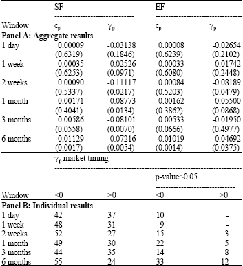 | |
| Analysis with Eq. 4 of market timing ability in Spanish equity mutual funds from July 1998 to September 2004. The difference Δβpt is the variation in the daily beta estimated by the Kalman filter. Market timing is evaluated by γp. Panel A shows the results for aggregate funds. SF (EF) is a size (equally) weighted portfolio made up of mutual funds in the sample. Panel B shows individual results. The p-value of each parameter is given in parentheses. The heteroskedasticity and autocorrelation consistent covariance estimator by Newey and West (1987) | |
In brief, these results would indicate that in general, mutual funds do not time the market in the short term. Only for a longer, 6 month period do 33 (14) funds out of 79% negative (positive) market timing. However, since managers’ timing decisions are not observable, caution should be exercised. The only firm conclusion is that for the 6 month window, the beta in 33 funds increased (decreased) when the market was down (up) while for 14, the opposite occurred. These changes in beta could be explained by factors other than market timing. Specifically, it is important to consider the effect of passive portfolio management in longer periods. Matallín and Fernández (2003) demonstrate how passive portfolios can show evidence of market timing in a simultaneous window when it is measured by the quadratic model. In the present case, if non-simultaneous timing is measured, the effect of passive management becomes greater as the window length increases. For example, suppose that a passive portfolio invests 50% in the stock index and 50% in T-Bills at the year beginning; thus the beta is 0.5. If the stock index achieves good (bad) results during the semester, the weight of the part invested in equities goes up (down) and the aggregate beta of the portfolio will be higher (lower) than 0.5.
| Table 2: | Mutual fund market timing with previously omitted benchmark |
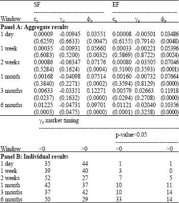 | |
| Analysis with Eq. 5 of market timing ability in equity Spanish mutual funds from July 1998 to September 2004. The difference Δβpt is the variation in the daily beta estimated by the Kalman filter. Market timing is evaluated by γp. The EMS is an equally-weighted benchmark which represents medium and small cap stocks. Panel A shows the results for aggregate funds. SF (EF) is a size (equally) weighted portfolio made up of mutual funds in the sample. Panel B shows individual results. The p-value of each parameter is given in parentheses. The heteroskedasticity and autocorrelation consistent covariance estimator is by Newey and West (1987) | |
Then this portfolio will evidence positive timing, because the beta has increased (decreased) when the market has been up (down). To shows this, we simulate passive portfolios that invest different weights in the IGBM stock index, the EMS benchmark and the risk free asset. Once 81 simulated buy-and-hold portfolios have been formed, returns are calculated and Eq. 5 is estimated for different windows. Table 3 shows the results and it is clear that for non-simultaneous windows, a buy-and-hold strategy generates evidence of positive market timing. Implicit increases (decreases) in the daily beta of the portfolio, resulting from the bull (bear) stock market in a wide window, imply a positive relation between market return and beta variation in this window.
A comparison of the results of Table 2 and 3 suggests that in general the mutual funds do not follow a buy-and-hold strategy and they rebalance their holdings to maintain a constant level of systematic risk. This is logical behaviour if the mutual fund wants to maintain a certain investment target. Consequently, mutual funds may show evidence of positive market timing in the long term if they follow a buy-and-hold strategy.
| Table 3: | Implicit timing in simulated passive portfolios |
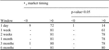 | |
| Analysis with (5) of market timing ability in simulated passive (buy-and-hold strategy) portfolios that invest, with different weights, in the IGBM stock index, the EMS benchmark and the risk free asset. Δβpt is the variation in the daily beta estimated by means of the Kalman filter. Market timing is evaluated by γp. The EMS is an equally-weighted benchmark which represents medium and small cap stocks. The p-value of each parameter is given in parentheses. The heteroskedasticity and autocorrelation consistent covariance estimator is by Newey and West (1987) | |
If mutual funds readjust beta, compensating implicit changes from a buy-and-hold strategy, the evidence will be of no market timing. However, if in this latter case managers’ decisions could be observed and only this information were considered, without taking into account implicit changes, the beta readjustment will lead to evidence of negative market timing. If mutual funds readjust beta in excess of the compensation for the implicit changes from the buy-and-hold strategy, negative market timing will be evidenced.
CONCLUSIONS
Mutual fund market timing is generally measured in a simultaneous window in the short term; in other words, the changes in beta over a brief period are compared with the market return at that moment. However, decisions on beta could affect subsequent periods; this is termed non-simultaneous timing. In the empirical study of a sample of Spanish mutual funds, the dynamic beta is estimated with the Kalman filter. Market timing is analysed by comparing changes in beta and market return. In the widest model, including a small and medium stocks benchmark, no evidence of timing is found in the simultaneous case. With larger windows, in the non-simultaneous case, the number of funds with positive and negative timing increases. However, in aggregate terms, no evidence of market timing is found for 1 week to 3 month windows. Only for the 6 month window is the evidence of negative timing greater. When this result is compared with that achieved by passive buy-and-hold portfolios, it seems that many mutual funds do not follow this strategy and that they time the market negatively in the long term.
ACKNOWLEDGMENTS
The author acknowledges the financial support provided by the Generalitat Valenciana grant GV/2007/097 and the financial support provided by Ministerio de Ciencia y Tecnología grant SEJ2007-67204/ECON.
REFERENCES
- Barone-Adesi, G., P. Gagliardini and G. Urga, 2004. Testing asset pricing models with coskewness. J. Bus. Econ. Statist., 22: 474-485.
Direct Link - Bollen, N.P.B. and J.A. Busse, 2001. On the timing ability of mutual fund managers. J. Finance, 56: 1075-1094.
CrossRefDirect Link - Brooks, R., R. Faff and M. Mckenzie, 1998. Time varying beta risk of Australian industry portfolios: A comparison of modelling techniques. Aust. J. Manage., 23: 1-22.
Direct Link - Ciriaco, A. and R. Santamari�a, 2005. Performance persistence of Spanish mutual funds. Investig. Econ., 29: 525-573.
Direct Link - Ferruz, L. and J. Sarto, 2004. An analysis of Spanish investment fund performance: Some considerations concerning sharpe's ratio. Omega, 32: 273-284.
Direct Link - Ferruz, L., I. Marco and J. Sarto, 2005. Performance in the management of Spanish and European investment funds. J. Applied Sci., 5: 988-998.
CrossRefDirect Link - Ferson, W. and R. Schadt, 1996. Measuring fund strategy and performance in changing economic conditions. J. Finance, 51: 425-461.
Direct Link - Goetzmann, W., J. Ingersoll and Z. Ivkovich, 2000. Monthly measurement of daily timers. J. Financial Quantitative Anal., 35: 257-290.
Direct Link - Harvey, C. and A. Siddique, 2000. Conditional skewness in asset pricing test. J. Finance, 55: 1263-1295.
Direct Link - Henriksson, R.D. and R.C. Merton, 1981. On market timing and investment performance. II. Statistical procedures for evaluating forecasting skills. J. Bus., 54: 513-533.
Direct Link - Holmes, K. and R. Faff, 2004. Stability, asymmetry and seasonality of fund performance an analysis of Australian multisector managed funds. J. Bus. Finance Account., 33: 539-578.
Direct Link - Koopman, S., N. Shephard and J. Doornik, 1999. Statistical algorithms for models in state space using SsfPack 2.2. Econ. J., 2: 113-166.
Direct Link - Marti�nez, M., 2003. Legal constraints, transaction costs and the evaluation of mutual funds. Eur. J. Finance, 9: 199-218.
Direct Link - Matall�n, J. and A. Fernandez, 2003. Passive timing effect in portfolio management. Applied Econ., 35: 1829-1837.
Direct Link - Matalli�n, J., 2005. Mixed portfolio management: The dynamics and timing between stocks and bonds. Int. J. Finance, 17: 3354-3375.
Direct Link - Matalli�n, J., 2008. The dynamics of mutual funds and market timing measurement. Studies Nonlinea Dyn. Econ. Forthcom.
Direct Link - Mckenzie, M., R. Brooks and R. Faff, 2000. The use of domestic and world market indexes in the estimation of time-varying betas. J. Multinat. Financial Manage., 10: 91-106.
Direct Link - Newey, W and D. West, 1987. A simple, positive semi-definite, heteroscedasticity and autocorrelation consistent covariance matrix. Econometrica, 55: 703-708.
Direct Link - Wells, C., 1996. The Kalman Filter in Finance, Advanced Studies in Theoretical and Applied Econometrics, 32. 1st Edn., Kluwer Academic Publishers, Dordrecht.
Direct Link