
M. Shakiba
Department of Electrical Engineering, KN Toosi University of Technology, Tehran, Iran
M. Teshnehlab
Department of Electrical Engineering, KN Toosi University of Technology, Tehran, Iran
S. Zokaie
Department of Electrical Engineering, KN Toosi University of Technology, Tehran, Iran
M. Zakermoshfegh
Department of Civil Engineering, Jundi-Shapur University of Technology, Dezful, Iran
Journal of Applied Sciences
Year: 2008 | Volume: 8 | Issue: 8 | Page No.: 1534-1540


ABSTRACT
In this study, a hybrid learning algorithm for training the Dynamic Synapse Neural Network (DSNN) to high accurate prediction of congestion in TCP computer networks is introduced. The idea behind this technique is to inform the TCP transmitters of congestion before it happens and to make transmitters decrease their data sending rate to a level which does not overflow the routers buffer. Traffic rate data are available in the format of time series and these real data are used to train and predict the future traffic rate condition. Hybrid learning algorithm aims to solve main problems of the Gradient Descent (GD) based method for the optimization of the DSNN, which are instability, local minima and the problem of generalization of trained network to the test data. In this method, Adaptable Weighted Particle Swarm Optimization (AWPSO) as a global optimizer is used to optimize the parameters of synaptic plasticity and the GD algorithm is used to optimize the weighted parameters of DSNN. As AWPSO is a derivative free optimization technique, a simpler method for the train of DSNN is achieved. Also the results are compared to GD algorithm.
PDF Abstract XML References Citation
How to cite this article
M. Shakiba, M. Teshnehlab, S. Zokaie and M. Zakermoshfegh, 2008. Short-Term Prediction of Traffic Rate Interval Router Using Hybrid Training of Dynamic Synapse Neural Network Structure. Journal of Applied Sciences, 8: 1534-1540.
DOI: 10.3923/jas.2008.1534.1540
URL: https://scialert.net/abstract/?doi=jas.2008.1534.1540
DOI: 10.3923/jas.2008.1534.1540
URL: https://scialert.net/abstract/?doi=jas.2008.1534.1540
INTRODUCTION
Due to traffic problems in router between Iran Telecommunication Research Center (ITRC) and Data Company, the aim of this study is prediction of interval traffic rate of that router (Box and Jenkins, 1976; Haltiner and Williams, 1980; Tanenbaum, 1996). One of the reasons of high rate of data loss in computer networks is the inability of the network to predict the congestion and inform the transmitters on time. The main objective of the study is introducing a powerful learning algorithm for training dynamic synapse neural network to high accurate prediction of chaotic time series. We monitored the traffic rate interval router in sampling of every thirty five minuets in December, January, February and March 2007 in kilo byte per second unit (Fig. 1). This time series has 5000 samples and we used 3000 samples for training and 2000 samples for testing neural network. We considered two learning algorithms for DSNN. These learning algorithms include the GD learning algorithm which uses GD for the training of both synaptic plasticity and weight matrix parameters and the hybrid learning algorithm which benefits both the PSO global search ability and the computational power of the GD. Finally some simulation results are provided for a comparison between these two methods.
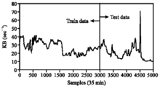 | |
| Fig. 1: | The real data for traffic rate during Dec., Jan., Feb. and Mar. 2007, with interval sample every 35 min |
MATERIALS AND METHODS
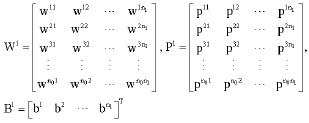
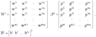
The structure of dynamic synapse neural network: Synaptic strength depends on three quantities: pre-synaptic activity xij(t); a use-dependent term Pij(t) which may loosely related to pre-synaptic release probability and postsynaptic efficacy Wij (Natschlager et al., 2001; Kim et al., 2003). Synaptic dynamics arise from the dependence of pre-synaptic release probability on the history of pre-synaptic activity. Specifically, the effect of activity xij(t) in the j-th pre-synaptic unit on the i-th postsynaptic unit is given by the product of the synaptic coupling between the two units and the instantaneous pre-synaptic activity as: xij(t).Pij(t).Wij(t). The pre-synaptic activity xij(t) is a continuous value (constrained to fall in the range [0, 1]). The coupling is in turn the product of a history-dependent release probability Pij(t) and a static scale factor Wij(t) corresponding to the postsynaptic response or potency at the synapse connecting j and i. Note that Wij≥0 for excitatory synapses and Wij≤0 for inhibitory synapses. The history-dependent component Pij(t) is constrained to fall in the range (0, 1). This component in turn depends on two auxiliary history-dependent functions fij(t) and dij(t). The quantity dij(t) can be interpreted as the number of releasable synaptic vesicles; it decreases with activity and thereby instantiates a form of use-dependent depression. The quantity fij(t) represents the propensity of each vesicle to be released; like (Ca2+) in the pre-synaptic terminal, it increases with pre-synaptic activity xj(t) and thereby instantiates a form of facilitation. fij(t) models facilitation (with time constant Fij>0 and the initial release probability Uij ∈ [0, 1]), whereas dij(t) models the combined effects of synaptic depression (with time constant Dij>0) and facilitation. Hence, the dynamics of a synaptic connection is characterized by the three parameters Uij ∈ [0, 1], Dij>0, Fij>0. For the numerical results presented in this paper we consider a discrete time (t = 1,2,...,T) version of the model defined by Eq. 1. In this setting we consider the dynamics with the initial conditions ![]() and dij(1) = 1. Note that in this case the time constants Fij and Dij have to be≥1 (Mehrtash et al., 2003; Kasthuri and Lichtman, 2004).
and dij(1) = 1. Note that in this case the time constants Fij and Dij have to be≥1 (Mehrtash et al., 2003; Kasthuri and Lichtman, 2004).
| (1) |
| (2) |
| (3) |
| (4) |
The input-output behavior of this model synapse depends on the four synaptic parameters Uij, Fij, Dij and Wij, as described, the same input yields markedly different outputs for different values of these parameters.
The dynamic synapses we have described (Fig. 2) are ideally suited to process signals with temporal structure.
Based on Fig. 2 we can show:
| (5) |
 | |
| Fig. 2: | Network architecture. The activation function at the hidden units was log-sigmoid function and linear function at the output unit |
 | (6) |
| (7) |
| (8) |
| (9) |
 | (10) |
| (11) |
| (12) |
Particle swarm optimization: Particle Swarm Optimization (PSO) was originally designed and introduced by Eberhart and Kennedy (1995) and Kennedy and Eberhart (1995, 2001). The PSO is a population based search algorithm based on the simulation of the social behavior of birds, bees or a school of fishes. This algorithm originally intendeds to graphically simulate the graceful and unpredictable choreography of a bird folk. A vector in multidimensional search space represents each individual within the swarm. This vector has also one assigned vector, which determines the next movement of the particle and is called the velocity vector. The PSO algorithm also determines how to update the velocity of a particle. Each particle updates its velocity based on current velocity and the best position it has explored so far and based on the global best position explored by swarm (Engelbrecht, 2005, 2002; Sadri and Suen, 2006). The PSO process then is iterated a fixed number of times or until a minimum error based on desired performance index is achieved. It has been shown that this simple model can deal with difficult optimization problems efficiently.
A detailed description of PSO algorithm is presented in (Eberhart and Kennedy, 1995; Kennedy and Eberhart, 1995, 2001). Here we will give a short description of the PSO algorithm proposed by Kennedy and Eberhart. Assume that our search space is d-dimensional and the i-th particle of the swarm can be represented by a d-dimensional position vector Xi = (x1i, x2i,...,xdi). The velocity of the particle is denoted by Vi = (v1i, v2i,...,vdi). Also consider best visited position for the particle is Pibest = (p1i, p2i,...,pdi) and also the best position explored so far is Pgbest = (p1g, p2g,...,pdg). So the position of the particle and its velocity is being updated using following equations:
| (13) |
| (14) |
where, c1 and c2 are positive constants and φ1 and φ2 are two uniformly distributed number between 0 and 1. In this equation, W is the inertia weight, which shows the effect of previous velocity vector on the new vector. The inertia weight W plays the role of balancing the global and local searches and its value may vary during the optimization process. A large inertia weight encourages a global search, while a small value pursues a local search. In (Mahfouf et al., 2004) authors have proposed an Adaptive Weighted PSO (AWPSO) algorithm in which the velocity formula of PSO is modified as follows:
| (15) |
The second term in Eq. 15 can be viewed as an acceleration term, which depends o n the distances between the current position xi the personal best pi and the global best pg. The acceleration factor α is defined as follows:
| (16) |
where, Nt denotes the number of iterations, t represents the current generation and the suggested range for α is (0.5, 1). As can be seen from Eq. 16, the acceleration term will increase as the number of iterations increases, which will enhance the global search ability at the end of run and help the algorithm to jump out of the local optimum, especially in the case of multi-modal problems. Furthermore, instead of using a linearly decreasing inertia weight, they used a random number, which was proved by Zhang and Hu (2003) to improve the performance of the PSO in some benchmark functions as follows:
| (17) |
where, is w0 ∈ (0, 1) a positive constant and r is a random number uniformly distributed in (0, 1). The suggested range for w0 is (0, 0.5), which makes the weight w randomly varying between 0 and 1. An upper bound is placed on the velocity in all dimensions. This limitation prevents the particle from moving too rapidly from one region in search space to another. This value is usually initialized as a function of the range of the problem. For example if the range of all xij is (-1, 1) then Vmax is proportional to 1.
pibest For each particle is updated in each iteration when a better position for the particle or for the whole swarm is obtained. The feature that drives PSO is social interaction. Individuals (particles) within the swarm learn from each other and based on the knowledge obtained then move to become similar to their better previously obtained position and also to their better neighbors. Individual within a neighborhood communicate with one other. Based on the communication of a particle within the swarm different neighborhood topologies are defined. One of these topologies which is considered here, is the star topology. In this topology each particle can communicate with every other individual, forming a fully connected social network. In this case each particle is attracted toward the best particle (best problem solution) found by any member of the entire swarm. Each particle therefore imitates the overall best particle. So, the pgbest is updated when a new best position within the whole swarm is found.
Learning algorithms for dynamic synapse neural network model: Here, two learning algorithms for the training of DS model are discussed.
GD based training of DSNN model: A minimizing of the sum of the square errors is used for training as the supervise rule:
| (18) |
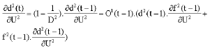
Here, we describe the basics of the conjugate gradient learning algorithm- a generalized version of simple gradient descent-which we used to minimize the MSE between the network Output y(n) in response to the input time series x(t) and the target output is d(n). In order to apply a conjugate gradient algorithm ones has to calculate the partial derivatives ![]() for all synapses < ij > in the network.
for all synapses < ij > in the network.
We state the equations for all of the partial derivatives for the network architecture shown in Fig. 2 (i.e., four dimensional network input and one-dimensional output and a single synapse between a pair of neurons). The calculations and determining the updates of Wij, Fij, Uij and Dij are started from outer layer. For calculating the partial derivatives ![]() we can show:
we can show:
| (19) |
| (20) |
| (21) |
| (22) |
 | (23) |
Similar calculations are needed for the optimization of other synaptic plasticity parameters. But the optimization rule for the weighted are quite simple and as follows:
| (24) |
To ensure that the parameters 0≤U≤1, D≥1, F≥1 and W≥1 (indices skipped for clarity) stay within their allowed range we introduce the unbounded parameters ![]() with the following relationships to the original parameters:
with the following relationships to the original parameters: ![]()
![]() . The conjugate gradient algorithm was then used to adjust these unbounded parameters which are allowed to have any value in R. The partial derivatives of E[y,d] with respect to the unbounded parameters can easily be obtained by applying the chain rule, e.g.,
. The conjugate gradient algorithm was then used to adjust these unbounded parameters which are allowed to have any value in R. The partial derivatives of E[y,d] with respect to the unbounded parameters can easily be obtained by applying the chain rule, e.g.,
| (25) |
As it was shown before, the learning rules for the parameters of the antecedent part are complex and cannot be easily calculated. Also, as it was mentioned before GD learning algorithm, suffers from some shortcomings that are mainly local minima problem, selection of the learning rate, stability problems and insensitivity to long-term dependencies.
Hybrid training of DSNN: The hybrid-learning algorithm proposed here uses Adaptable Weighted Particle Swarm Optimization (AWPSO) based method to train the parameters of synaptic plasticity (U, F, D) and GD based methods for tuning the weights. These methods provide derivative free exploration for solution in input space. In addition using hybrid algorithms less local minimum solutions may be obtained.
The components of each particle in PSO population are (Uij, Fij, Dij) parameters. The update rules of each population are as Eq. 14-17, which is the update rule for AWPSO. In this algorithm in each step the PSO will update the Uij, Fij, Dij parameters between all layers and then the GD optimizer will run once to update the weights parameters using train data and the update rule for the weights parameters. After update of the parameters of both Wij and Uij, Fij, Dij, one epoch has completely performed and mean squared error of the train data is calculated. This value would be the cost function of each particle which must be minimized. For a better exploration of the search space a mutation operator is defined. The previous vector of velocity in this way is reset to a random vector if for some iteration the global best value doesn’t change.
RESULTS AND DISCUSSION
The simulations are presented here to compare the hybrid learning algorithm and the gradient descent learning algorithm. The simulations include time series prediction and identification of interval traffic rate router.
One hundred epochs for each algorithm was chosen and the best epoch for them was chosen within 500 epoch of run of algorithms. The best epoch chosen here, is the epoch after which the error for test data becomes larger. In addition to have a better comparison both algorithms run for 10 times.
| Table 1: | Comparing methods for prediction of interval traffic rate router |
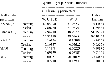 | |
As it can be seen the hybrid algorithm returns much better results in terms of generalization in testing and training (Table 1). In addition the results obtained by hybrid training algorithm are very near together. This result shows that independent of the initial population the results of hybrid algorithm will always converge to almost same point and the results are much more reliable than the GD algorithm. Also as it is shown the results obtained by hybrid learning algorithm proposed here are better.
The results of using GD learning algorithm: In Fig. 3, we use four-dimensional network input, one-dimensional network output and two hidden layers with towel neurons in first layer and six neurons in second layer. With this structure the network has 504 learning parameters. The standard deviation of Fitness of GD learning algorithm for test data is 22.3127%.
We compared network performance when different parameter subsets were optimized using the conjugate gradient algorithm, while the other parameters were held fixed. In all experiments, the fixed parameters were chosen to ensure heterogeneity in pre-synaptic dynamics. To achieve better performance one has to change at least two different types of parameters such as {W, U} or {W, D} (all other pairs yield worse performance) (Fig. 4). The standard deviation of Fitness of GD learning algorithm for test data is 28.0365%. The results of changing {W, U} are as follows:
The results of using hybrid learning algorithm: To improve exploration ability of the PSO small value for maximum velocity is selected. This value in all of experiments is 0.2. Also the values of w0 is 0.5 and the value of α0 is 1. The population size of the PSO for all of the experiments is 20. In simulations we use two-dimensional network input, one-dimensional network output and one hidden layer with towel neurons. With this structure the network has 144 learning parameters. In Fig. 5 the standard deviation of Fitness of hybrid learning algorithm for test data is 88.3042%.
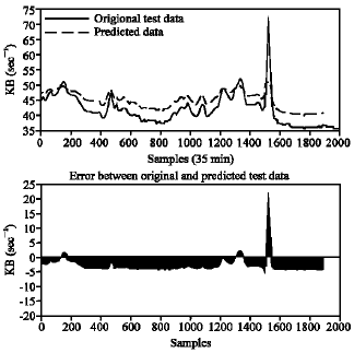 | |
| Fig. 3: | One step ahead prediction of traffic rate time series with all of the learning parameters (Wij, Fij, Uij, Dij) |
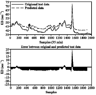 | |
| Fig. 4: | One step ahead prediction of traffic rate time series with two learning parameters (Wij, Uij) |
Know the results are presented here to compare the hybrid learning algorithm and the gradient descent learning algorithm. For evaluating and comparing two different modeling and prediction methods which have been examined, five criteria are considered.
| • | Root Mean Squared Errors (RMSE) |
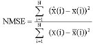
| • | Normalized Mean Squared Errors (NMSE) |
| • | Mean Absolute Error (MAE) |
| • | Mean Bias Error (MBE) |
| • | Fitness (100-NMSE) |
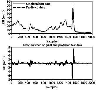 | |
| Fig. 5: | One step ahead prediction of traffic rate by DSNN (two dimensional network input, one-dimensional network output and one hidden layer with towel neurons) |
The criteria are defined as:
| (26) |
where, x is the measured and x̂ is the Predicted value.
 | (27) |
where, the value of x is the mean of the measured data.
| (28) |
| (29) |
CONCLUSION
In this study, a hybrid learning algorithm for DSNN model has been introduced. The hybrid method introduced, uses AWPSO for the training of the parameters of synapses and the GD algorithm to optimize the weighted parameters of the DSNN. This method was compared with GD learning algorithm which uses GD algorithm to optimize both the parameters of synapses and weights. The GD algorithm suffers from some shortcomings which are mainly stability problems, complexity of learning algorithm, sensitivity to initial conditions of the values, local minima problems and the problem of overtraining to the train data. As it was shown before using the hybrid algorithm different initial conditions for parameters will converge to almost the same point and less local minima problem may occur. Also generalization results were quite better and less stability problems may happen. The simulation results support these complain. In addition, by using hybrid learning algorithm, the learning rules of the parameters simple.
ACKNOWLEDGMENTS
The authors would like to express their gratitude to Iran Telecommunication Research Center for their support and consent.
REFERENCES
- Bowker, R.M., S.J. Rockershouser and K.B. Vex, 1993. Immunocytochemical and dye distribution studies of nerves potentially desensitized by injections into the distal interphalangeal joint or the navicular bursa of horses. J. Am. Vet. Med. Assoc., 203: 1708-1714.
Direct Link - Bowker, R.M., K. Linder and I.M. Sonea, 1995. Sensory innervation of the navicular bone and bursa in the foal. Equine Vet. J., 27: 60-65.
Direct Link - Dyson, S.J. and L. Kidd, 1993. A comparison of responses to the analgesia of the navicular bursa and intra-articular analgesia of the distal interphalangeal joint in 59 horses. Equine Vet. J., 25: 93-98.
Direct Link - Gibson, K., C. McIlwraith and R. Park, 1990. A radiographic study of the distal interphalangeal joint and navicular bursa of the horse. Vet. Radiol., 31: 22-25.
Direct Link - Gough, M.R., I.G. Mayhew and G.A. Munroe, 2002. Diffusion of mepivacaine between adjacent synovial structures in the horse. Part 1: Forelimb foot and carpus. Equine Vet. J., 34: 80-84.
Direct Link - Pleasant, R.S., H.D. Moll and W.B. Ley, 1997. Intra-articular anesthesia of the distal interphalangeal joint alleviates lameness associated with the navicular bursa in horses. Vet. Surg., 26: 137-140.
Direct Link - Sack, W.O., 1975. Nerve distribution in the metacarpus and front digit of the horse. J. Am. Vet. Med. Assoc., 167: 298-305.
Direct Link - Sardari, K., H. Kazemi and M. Mohri, 2002. Effects of analgesia of the distal interphalangeal joint and navicular bursa on experimental lameness cause by solar pain in horses. J. Vet. Med., A49: 478-481.
Direct Link - Schumacher, J., R. Steiger, J. Schumacher, F. Graves, M. Schramme, R. Smith and M. Coker, 2000. Effects of analgesia of the distal interphalangeal joint or palmar digital nerves on lameness caused by solar pain in horses. Vet. Surg., 29: 54-58.
Direct Link - Schumacher, J.O., J.I. Schumacher and F. De Graves, 2001. A comparison of the effects of local analgesic solution in the navicular bursa of horses with lameness caused by solar toe or solar heel pain. Equine Vet. J., 33: 386-389.
Direct Link - Schumacher, J.O., J.I. Schumacher and R. Gillette, 2003. The effects of local anaesthetic solution in the navicular bursa of horses with lameness caused by distal interphalangeal joint pain. Equine Vet. J., 35: 502-505.
Direct Link - Schramme, M.C., J.C. Boswell and K. Hamhoughias, 2000. An in vitro study to compare 5 different techniques for injection of the navicular bursa in the horse. Equine Vet. J., 32: 263-267.
Direct Link - Turner, T.A., 1989. Diagnosis and treatment of navicular syndrome in horses. Vet. Clin. N. Am. Equine Pract., 5: 131-144.
Direct Link