
L. Zjavka
Department of Informatics, Faculty of Management Science and Informatics, University of �ilina, Univerzitn� 8215/1, 010 01, �ilina, Slovakia
Journal of Artificial Intelligence
Year: 2011 | Volume: 4 | Issue: 1 | Page No.: 89-99


ABSTRACT
Artificial neural network identification in general is based on pattern similarity and absolute values of input variables, but these can differ enormously while their relations may be the same. Generalization (learning) of these dependencies could be a way of modelling systems more similar to human brain learning than a pattern classification. Differential polynomial neural network is a new type of neural network developed by author, which constructs a differential equation, describing system of dependent variables. It creates derivative fractional terms defining a mutual change of some input variable combinations. Its response should be the same to all input patterns, which variables behave the trained dependence (regardless of their values). The most important function of brain seems to be a generalization of received information, i.e., forming ideas of common validity from received data. How does a biological neural cell process information and how it functionality essentially differs from artificial neuron ? It seems to create some polynomial multi-parametric functions, which could be better modeled by polynomial neuron. It should describe the partial dependence of some combinations of variables, using a special type of simple polynomial functions. However neural cell applies periodic activation function to create derivative terms of which differential equation describing data relations consists.
PDF Abstract XML References Citation
How to cite this article
L. Zjavka, 2011. Differential Polynomial Neural Network. Journal of Artificial Intelligence, 4: 89-99.
DOI: 10.3923/jai.2011.89.99
URL: https://scialert.net/abstract/?doi=jai.2011.89.99
DOI: 10.3923/jai.2011.89.99
URL: https://scialert.net/abstract/?doi=jai.2011.89.99
INTRODUCTION
Artificial Neural Networks (ANN) in general identify patterns according to their relationship, responding to related patterns with a similar output. They are trained to classify certain patterns into groups and then are used to identify the new ones, which were never presented before. If ANN is trained for instance to identify a shape, it can correctly classify only incomplete or similar patterns as compared to the trained ones were (Marcek and Marcek, 2006). But in case a shape is moved or its size is changed in the input matrix of variables the neural network identification will fail. The principal lack of the ANN identification in general is the disability of input pattern generalization. ANN is in principle a simplified form of polynomial neural network (PNN), which combinations of variables are missing. Polynomial functions apply those to preserve partial dependencies of variables. That’s why the ANN’s identification can’t utilize data relations (including time-series prediction), which are described lots of complex systems (Zjavka, 2007).
Let’s try to look at the vector of input variables as a no pattern but bound dependent point set of N-dimensional space. Likewise the ANN pattern classification works, we can reason an identification of any unknown relations of the input data variables. The neural network response would be the same to all patterns (dependent sets), which variables behave the trained dependence. It doesn’t matter what values they become. A multi-parametric non-linear function can describe this relation to each other. So if we want to create such a function with neural network, its neurons must apply some n-parametric polynomial functions to catch the partial dependence of its n-inputs. Biological neural cell seems apply a similar principle. Its dendrites collect signals coming from other neurons. But unlike the ANNs the signals interact already in the single branches (dendrites) likewise the variables of a multi-parametric polynomial. So, this could be modelled with multiplications of some inputs in polynomials of PNN. Then these weighted combinations are summed in the cell body and transformed using time-delayed dynamic periodic activation function (activated neural cell generates in response to its input signals series of time-delayed output pulses) (Benuskova, 2002). The period of this function depends on some input variables and seems to represent the derivative part of a partial derivation of an entire polynomial (as a term of differential equation).
Polynomial neural network for dependence of variables identification (or Differential polynomial neural network - D-PNN, because it constructs a differential equation) describes a functional dependence of input variables (not entire patterns as ANN does). This could be regarded as a pattern abstraction, similar the brain utilizes, which identification is not based on values of variables but only relations of these. D-PNN forms its functional output as a generalization of input patterns.
GMDH POLYNOMIAL NEURAL NETWORK
General connection between input and output variables is expressed by the Volterra functional series, a discrete analogue of which is Kolmogorov-Gabor polynomial (Ivakhnenko, 1971):
| (1) |
Where:
| m | : | No. of variables |
| X(x1, x2,. .., xm) | : | Vector of input variables |
| A(a1, a2,. .., am),. .. | : | Vectors of parameters |
This polynomial can approximate any stationary random sequence of observations and can be computed by either adaptive methods or system of Gaussian normal equations (Ivakhnenko, 1971).
The starting point of the new neural network type D-PNN development was the GMDH polynomial neural network, created by a Ukrainian scientist Aleksey Ivakhnenko in 1968. When the back-propagation technique was not known yet a technique called Group Method of Data Handling (GMDH) was developed for neural network structure design and parameters of polynomials adjustment. He attempted to resemble the Kolmogorov- Gabor polynomial (1) by using low order polynomials Eq. 2 for every pair of the input values (Galkin, 2000):
| (2) |
The GMDH neuron (Fig. 1) has two inputs and its output is a quadratic combination of 2 inputs, total 6 weights. Thus GMDH network builds up a polynomial (actually a multinomial) combination of the input components. Typical GMDH network (Fig. 2) maps a vector input x to a scalar output y', which is an estimate of the true function f(x) = y. Each neuron of the polynomial network fits its output to the desired value y for each input vector x from the training set.
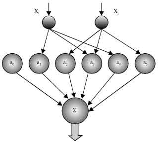 | |
| Fig. 1: | GMDH polynomial neuron |
 | |
| Fig. 2: | GMDH polynomial neural network |
The manner in which this approximation is accomplished is through the use of linear regression (Galkin, 2000).
In the hope to capture the complexity of a process, this neural network attempts to decompose it into many simpler relationships each described by a processing function of a single neuron (2). It defines an optimal structure of complex system model with identifying non-linear relations between input and output variables. Polynomial Neural Network (PNN) is a flexible architecture, whose structure is developed through learning. The number of layers of the PNN is not fixed in advance but becomes dynamically meaning that this self-organising network grows over the trained period (Oh et al., 2003).
GENERALIZATION OF PATTERNS
Let’s consider an ANN trained to identify a shape. It can correctly identify only incomplete or similar patterns as compared to the trained one, activating the same areas of neurons. But in a case the shape is moved or its size is changed in the input matrix, it will seem to the ANN to be an entirely new pattern.
 | |
| Fig. 3: | Characteristic points of a changeable pattern |
A way to be solved this problem is to define several characteristic points of the pattern (decomposition of a shape forming the input vector) and try D-PNN to learn their dependences. These relations define non-linear multi-parametric functions, creating by multiplications (combinations) of input variables of polynomials, applied to general pattern identification (Zjavka, 2010).
You can see, that the condition of the significant point pattern dependence of a rectangle (Fig. 3) is defined by equal x-coordinates of the points Ax = Bx and Cx = Dx and corresponding y-coordinates Ay = Cy and By = Dy. Another more complicated diagonal dependence applies the x,y-coordinates of the points A,D and C,B to oblique square determination. There will have to equal their x and y-position difference Ax-Ay = Dx-Dy and sum Cx+Cy = Bx+By. D-PNN recognises the square shape in this 2-way mannered dependence. This corresponds with recent human brain researches, which proved recognizing shapes are decomposed into several elementary elements, activating some biological neural cells as characteristic marks of a pattern. Human brain does not utilize absolute input values but relative reciprocal ones, creating by periodic dynamic functions of biological neurons (Benuskova, 2002).
DIFFERENTIAL POLYNOMIAL NEURAL NETWORK
The basic idea of the author’s D-PNN is to approximate a differential Eq. 3, which can define relations of variables (Hronec, 1958), with a special type of root fractional polynomials - for instance Eq. 4-5.
| (3) |
Where:
| u = f(x1, x2,, …, xn) | : | Function of input variables |
| a, B(b1, b2,,. .., bn), C(c11, c12,,. ..) | : | Parameters |
Elementary methods of the common Differential Equation (DE) solution express the solution in special elementary functions - polynomials (such as Bessel’s functions or power series). Numerical integration of differential equations is based on an approximation of these using:
| • | Rational integral functions |
| • | Trigonometric series |
I have selected the 1st more simple way using method of integral analogues, by replacing mathematical operators in equations with ratio of pertinent values (Kunes et al.,1989).
 | (4) |
 | (5) |
Where:
| n | : | Combination degree of n- input variables of numerator |
| m | : | Combination degree of denominator (m<n) |
The fractional polynomials Eq. 4, which describe a partial dependence of n-input variables of each neuron, are applied as terms of DE Eq. 3 construction. They partly create an unknown multi-parametric non-linear function, which codes relations of variables. The numerator of equation Eq. 4 is a polynomial of complete n-input combinations of a single neuron and realizes a new function z of formula Eq. 6. The denominator of Eq. 4 is a derivative part, which gives a partial mutual change of certain neuron input variables and its polynomial combination degree m is less then n. It is arisen from the partial derivation of the complete n-variable polynomial by competent variable(s). In general it is possible this approximation express in formula Eq. 6 (Hronec, 1958).
| (6) |
Where:
| z | : | Function of n-input variables |
| wi | : | Weights of terms |
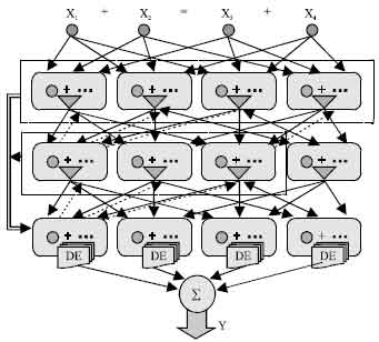
Each layer of the D-PNN consists of blocks of neurons (Fig. 4). Block contains derivative neurons, one for each fractional polynomial (4) of a derivative combination of variables. Inputs of constant combination degree (n = 2,3,…) forming certain combination of variables, enter each block, where they are substituted into polynomials of neurons. The final function Eq. 6 is formed in each block of the last hidden layer the D-PNN, which polynomials look like the formula Eq. 5. The root functions of denominators Eq. 5 are lower then n, according to their combination degree and take the polynomials of neurons into competent power degree. Blocks of other hidden layers consist of partial derivations (forming by neurons), which describe the input variable partial dependence Eq. 4.
 | |
| Fig. 4: | Differential polynomial neural network |
Their neurons don’t affect the block output but are applied only for total output calculation by the DE composition (using root functions in blocks of the last hidden layer). Each block also contains a single polynomial (without derivative part), which forms its output entered the next hidden layer of the network Each neuron has 2 vectors of adjustable parameters a, b and each block consists 1 vector of adjustable parameters of single polynomial. There it is necessary to adjust not only polynomial parameters, but the D-PNN‘s structure too. This means some neurons in role of terms of the DE have to be left out.
IDENTIFICATION OF DEPENDENCIES OF VARIABLES
Consider a very simple dependence of 2-input variables, which difference is constant (for example = 5). D-PNN will learn this relation easily according to training data set by means of Genetic Algorithm (GA).
 | (7) |
D-PNN will contain only 1 block of 1 polynomial neuron Eq. 7 as a term of DE (Fig. 5). As the input variables are changing constantly, there is not necessary to add the 2nd term (fractional polynomial of derivate variable x2) in the DE (block), which causes occasional output mistakes by identification. Another example can solve 2 inputs, where the multiplicity of the inputs is constant (Fig. 5).
The input variables are not changing constantly, so there will be necessary both terms of the DE - fractional polynomial of derivative variable x2 too Eq. 8:
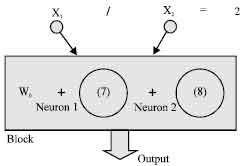 | |
| Fig. 5: | Identification of a constant quotient of 2 variables (x1 = 2x2) |
 | |
| Fig. 6: | Relations of chess pieces |
 | (8) |
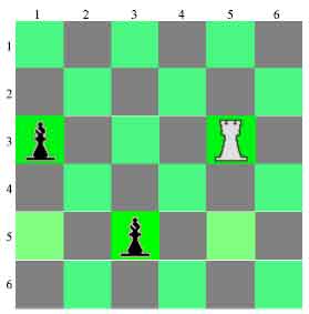
Simple D-PNN composed of these 4 blocks (one block for each pair of input variables) can learn the characteristic point dependence of a rectangle (Fig. 3). If x and y-coordinates of lined points equal, their difference = 0 and D-PNN can identify this. The 2-variable blocks also can solve another example, which shows the dependence of chess pieces (Fig. 6). Input of the neural network is formed by their x and y-positions. If the white rook checks the black bishop (their x or y positions equal) the 2-variable dependence comes true.
Dependence of the oblique square is defined through the diagonal coordinates of its characteristic points (Fig. 3). If difference and sum of the x and y-positions of diagonal points equal, the oblique square dependence condition comes true. This can solve D-PNN consisting of 2 blocks of 4 input variables (Fig. 7). Likewise the chess example shows a diagonal dependence of pieces, if the black bishop checks the white rook (Fig. 6). This can learn again one 4-variable block.
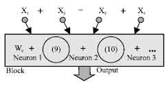
There are totally 14 combinations (neurons) of 4 input variables, for all derivative terms (1,2,3-combinations) of DE in the block. Some of them have to be taken off, as cause the D-PNN will work amiss. Each DE term also has an adjustable weight wi. Neurons can form for example the fractions Eq. 9-10:
 | |
| Fig. 7: | Identification of dependencies of 4 variables |
 | (9) |
 | (10) |
D-PNN as well is charged by possible 2-sided dependence change of input variables. For example 1+9 = 10 is the same sum as 9+1 = 10. Some mistakes can occur by identification, if GA adjustment finishes in a local error minimum. However it can be clearly seen that the D-PNN operates. If the sum of the 1st pair of variables is less then the 2nd one, the output of the D-PNN is less than desired and the other hand round. So there is shown a separating plane detaching relative classes, which are the same characteristic likewise it is current by ANN’s pattern identification.
MULTI-LAYERED D-PNN
Multi-layered D-PNN with 2 or 3-combination blocks can also solve previous examples. For simplicity we construct first the D-PNN for the 3-variable sum dependence identification (Fig. 8). The problem of the multi-layered D-PNN construction reside in that we try to create every partial combination term of a complete DE utilizing some fixed lower combination degree (2, 3) of blocks, while the amount of input variables is higher.
Each executable block of the last hidden layer takes part in the total network output calculation (creates its own DE) utilising its own neurons and back neurons of connected blocks the previous layers (Fig. 8). Blocks of other hidden layers create its output using single adjustable polynomial without derivative part (p = polynomial on Fig. 8), but their neurons are applied only for the total DE composition (in blocks of the last hidden layer). First the blocks of the last hidden layer take its own neurons as 2 basic terms (11) of the DE (6). Subsequently they create 4 terms of the 2nd (previous) hidden layer, using neurons and polynomials of bound blocks. They join these 2 blocks and create 4 fractional terms of the DE utilising 4 derivate variables (of 2 previous blocks) for instance Eq. 12.
 | (11) |
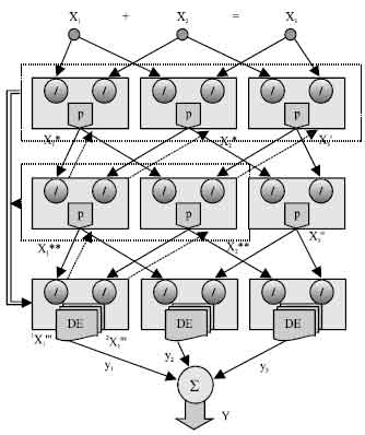 | |
| Fig. 8: | Identification of the 3-variable sum dependence with 2-variable combination blocks |
 | (12) |
 | (13) |
The backward connection of the previous layer(s) is realized through polynomials of the linked 2nd (or 1st) layer blocks. These are directly creating derivative part in numerator of formulas Eq. 12-13. Likewise we can create terms of the 1st hidden layer Eq. 13. We attach all its 3 linked blocks, forming 6 terms of the DE (1 duplicated connection is not used). The multiplication 2* in denominators of formulas Eq. 11-13 is used to decrease the D-PNN total output value. There is not used every term of all 12 terms of the complete DE, some of them have to be eliminated. This indicates 0 or 1 for each term in the executable blocks of the last hidden layer (creating DE) and are ease to use as genes of GA adjustment (Obitko, 1998). Parameters of polynomials are represented by real numbers. A chromosome is a sequence of their values, which can be easy mutated. The searching space probably contains a great amount of local error solutions, which GA can finish easily. The advantage of D-PNN adjustment is using only small training data set (likewise the GMDH PNN does), to learn any dependence.
 | |
| Fig. 9: | 3-variable combination block D-PNN |
The 3-variable combination block D-PNN of 4 input variables will have 3 hidden layers, each consisting of 4 blocks (for each 3-combination), to reach back all the 1st layer input variables from the last layer executable blocks (Fig. 9). Each block consists of 6 neurons (partial derivations) of all its 1 and 2-combinations. Likewise the previous D-PNN type (Fig. 8) we can construct the partial fractional terms of the DE (for each block of the last hidden layer) from back-connected neurons of previous layers. There is possible to apply only some of the connection parts of fractions. We can also construct the 4 dependent input variable D-PNN using 2-combination blocks. There will be 6 blocks of all input combination couples in the 1st hidden layer and consequently the number of them is increasing each next layer. D-PNN totally will consist of 6 hidden layers of blocks. Some problems can cause the composition of derivative terms from fractions because a lot of input combinations may rise and have to be tested. There might be suitable apply some methods of genetic programming to more accurate DE construction especially if D-PNN contains plenty of input variables.
CONCLUSION
D-PNN is a new neural network type designed by author, which can learn to identify any unknown dependencies of data set variables (not entire patterns as the ANNs do). It doesn’t utilize absolute values of variables but relative ones, likewise the brain does. This identification could be regarded as a pattern abstraction (or generalization), similar human brain utilizes according to data relations. But it applies the approximation with time-delayed periodic activation functions of biological neurons in high dynamic system of behaviour (Benuskova, 2002). D-PNN constructs a differential equation, which describes a system of dependent variables, with rational integral polynomial functions. Instead of these some periodic functions could be used (sin, cos) for this operation (Fig. 10) (Kunes et al.,1989). Changeable periods ω will replace the derivative parts (denominator) of equations e.g., Eq. 7-8 in this case Eq. 14-15. Activation functions (e.g., sigmoid) of artificial neuron seem to be periodic functions too, but their period ω = ∞. So, this might be a special case (applying by ANN) of common periodic function (Zjavka, 2008). The problem of the D-PNN construction resides in the method of the partial DE term composition of all possible combinations and how the partial derivative (dependence) of some input variables is realized (through fractional or periodic functions).
 | |
| Fig. 10: | Transformation of absolute values of variables using periodic function |
| (14) |
| (15) |
Relations of some data variables describe a lot of complex systems. D-PNN could model their behaviour, for example the weather prediction could be based on many unknown generalized relations of the data (such as pressure, temperature, etc.) instead of time-series prediction utilising pattern identification.
REFERENCES
- Ivakhnenko, A.G., 1971. Polynomial theory of complex systems. Proceedings of the IEEE Transactions on Systems, Oct. 1971, Institute of Electrical and Electronics Engineers, Inc., pp: 364-371.
Direct Link - Oh, S.K., W. Pedrycz and B.J. Park, 2003. Polynomial neural networks architecture: Analysis and design. Comput. Electrical Eng., 29: 703-725.
CrossRef - Zjavka, L., 2010. Generalization of patterns by identification with polynomial neural network. J. Electrical Eng., 61: 120-124.
Direct Link