
Abdallah Hage Hassan
Department of Mechanical Engineering, Oakland University, Rochester, MI, 48309-4401, USA
Asian Journal of Applied Sciences
Year: 2014 | Volume: 7 | Issue: 5 | Page No.: 273-293


ABSTRACT
Vibratory stress relief is a process used to relief residual stresses in mechanical components such as castings and welded parts by mean of vibration or cyclic loading. Some studies claimed that vibratory stress relief is effective while others deny these claims. It seems that this process is not fully understood. This study was done to understand cyclic loading and its effects on relieving residual stresses in mechanical components. Analysis on a cantilevered beam was done to come up with a model to predict the remaining residual stress after applying cyclic loading.
PDF Abstract XML References Citation
Received: October 19, 2013;
Accepted: April 14, 2014;
Published: May 05, 2014
How to cite this article
Abdallah Hage Hassan, 2014. Vibratory Stress Relief Analysis. Asian Journal of Applied Sciences, 7: 273-293.
DOI: 10.3923/ajaps.2014.273.293
URL: https://scialert.net/abstract/?doi=ajaps.2014.273.293
DOI: 10.3923/ajaps.2014.273.293
URL: https://scialert.net/abstract/?doi=ajaps.2014.273.293
INTRODUCTION
Welding, casting and other manufacturing processes create residual stresses within the surface of the part. Residual stresses are known to cause problems when combined with service load stresses. A process called Vibratory Stress Relief (VSR) is used to reduce these residual stresses. This process is known to have many advantages over other processes such as annealing but it is not fully understood. Throughout the year a substantial amount of work was done in this area such as: vibration of marine steel shaft with positive results on reducing micro residual stresses (Sun et al., 2004a), decreasing residual stresses on welded parts by 25% (Sun et al., 2004b), Vibratory Weld Conditioning (VWC) on welded body valves (Xu et al., 2007; Qinghua et al., 2008), cyclic loading on stainless steel welded parts proved effectiveness (Rao et al., 2007), computer simulation for vibrator stress relief by mean of cyclic loading proved that time has no effect on residual stress relief (Zhao et al., 2008) and cyclic loading extended the life of fatigue tests (Tuegel and Brooks, 1997).
None of the previous works found a mathematical model to explain the phenomenon of residual stress relief under cyclic or dynamic loading. The present work studied the fundamentals of cyclic loading such as stress controlled and strain controlled functions to understand their effect on residual stress reduction and distribution while performing vibratory stress relief. Cycle dependent hardening of the material and the Bauschinger effect are studied in detail. Distribution of residual stress in a rectangular bar after bending is analyzed based on superimposing an applied load and its inverse. Finally, the presented model can be used to predict residual stress relief using VSR.
CYCLIC LOADING
In essence there are two important aspects to the understanding of material behavior during the vibratory stress relief process (Sandor, 1972). First, a complete knowledge of the cyclic loading conditions imposed on the material is necessary. On a large scale this is normally not a difficult task but in some cases, such as those with complex geometry, the problem becomes difficult. Second, it must be realized that every material has its own way to respond to a particular imposed condition. In general material response to a specific loading is not constant from cycle to cycle. The two extremes of the changing response are cycle-dependent hardening and softening.
Stress controlled cyclic function: The possible responses of the material range between the two extremes shown in Fig. 1a-f. The controlled function has constant amplitude, σa Fig. 1a. The independent variable, strain, has the same frequency as the imposed load but its amplitude is not a constant. In the case of cycle-dependent hardening Fig. 1b, the material resistance to deformation increases from cycle to cycle so that the strain becomes smaller and smaller under the same stress. Cycle-dependent softening is a gradually decreasing resistance to deformation, Fig. 1c. It will be shown later that material hardening or softening are expected to occur in the first few cycles, after that a steady state is reached.
Strain controlled cyclic function: Again the controlled function has constant amplitude, εa Fig. 1d. The independent variable, stress, changes under exponential envelopes in both extremes shown. Cycle dependent hardening (Fig. 1e) means that the resistance to deformation increases so that larger and larger stresses are required to push and pull the material to the unchanging strain limits.
 | |
| Fig. 1(a-f): | Cycle-dependent material responses under stress and strain control, (a) Controlled function, stress (b) Cycle-dependent hardening; independent variable, strain (c) Cycle-dependent softening; independent variable, strain (d) Controlled function, strain (e) Cycle-dependent hardening; independent variable, stress and (f) Cycle dependent softening; independent variable, stress |
Cycle dependent softening makes the material deform more easily. Under strain control, therefore, the stress needed to enforce the strain limits becomes smaller and smaller as cycling progresses (Fig. 1f).
Hysteresis loop with cycle dependent hardening: Using ASTM A36 steel in previous experiments and given that steel may strain harden in cyclic loading, it is important to look at the stress strain diagram for the first few cycles. Vertical dotted lines are used to show strain control for different cycles (Fig. 2). The successive numbers represent the stress levels at which the strain limits are reached as cycling progress. Since, hardening means an increasing resistance to deformation, the stress required to push and to pull the material from one strain limit to the other gradually increases. The unloading from each loop tip is along the elastic slope so that the plastic strain per cycle is decreasing with successive cycles.
BAUSCHINGER EFFECT
If a metallurgically stable metal has been loaded, unloaded and then the stress is increased to a level that will cause plastic strain again, plastic flow occurs more easily than if unloading had not occurred that is, more easily than if the prior deformation had been continued without interruption (Lubhan and Felgar, 1961). The difference in behavior with and without interruption may be very large or very small, depending on the temperature, the amount of strain prior to the interruption and the direction of strain after interruption relative to the direction of the prior strain. The difference is particularly large when the direction of strain is reversed and it was under these conditions that the effect was first observed by Bauschinger (1886). The very low deformation resistance in one direction following prestraining in the opposite direction is called the “Bauschinger effect” (Lubhan and Felgar, 1961).
Effects under repeated reverse loading: After the stress has been reversed many times, the effects are simpler because a steady state develops wherein the effects do not change very much from one cycle to another. Both Ludwik and Scheu (1923) and Sachs et al. (1948) have shown that the stress-strain curve does not change appreciably with number of cycles after the first few cycles.
 | |
| Fig. 2: | Stress vs. strain for strain control and cycle-dependent hardening |
The number of cycles required before a steady state condition prevails depends on the plastic strain per cycle. When the plastic strain per cycle is quite small, three or four cycles may be required. For large values of plastic strain per cycle, the curves for all cycles after the first may be the same. Sachs et al. (1948) have done tests on the aluminum alloy 24ST in tension and compression. In these tests the plastic strain per cycle was maintained constant and the variation of stress with number of cycles was observed. For a large plastic strain per cycle there was a rapid approach to steady state conditions. Ludwik and Scheu (1923) found similar effects. When the maximum stress per cycle was held constant, the plastic strain per cycle diminished within the first few cycles to a value that remained constant nearly to failure.
In both Sachs’ and Ludwik’ work, the steady state situation that was established after the first few cycles prevailed up until near the time of fatigue failure. Then the metal began to soften: At constant plastic strain per cycle (Sachs) the maximum stress began to diminish and at a constant maximum stress (Ludwik) the plastic strain per cycle began to increase. In Ludwik tests, for example, the loops began to broaden out perceptibly at about 215 cycles out of 230 cycles to failure.
Reduction in residual stress after reversed bending: When a reversed bending load is superimposed on a certain residual stress distribution, one of the following two cases should occur:
| • | When σflow (the stress which is greater or equal to the yield stress) is not exceeded, unloading is elastic and no change in residual stress occurs |
| • | When σflow is exceeded the resulting effect is shown in Fig. 4 and plotted in the loop FGAH in Fig. 3. An example of an initial residual stress is plotted at F in Fig. 3 and is indicated by 1 in Fig. 4. The load stress is shown by FG in Fig. 3 and by the dashed line in Fig. 4. The maximum value of stress (the sum of the initial residual stress and the alternating load stress) that would exist if plastic flow did not occur is represented by the point G in Fig. 3 and by the right hand ordinate in sketch 2 of Fig. 4. Since, this maximum stress is greater than the yield strength, plastic flow will occur and the stress distribution will change in the manner indicated in sketch 3 of Fig. 4 |
The corresponding changes in strain are indicated in Fig. 5a-b. At the right side of the beam the compressive stress increases from its initial value (point 1, Fig. 5a) to the yield strength. Since, the corresponding elastic strain is less than the fixed strain limit imposed on account of the given nominal stress amplitude, the difference will be made up by plastic strain. This plastic strain occurs at the yield strength and results in conditions indicated by point 3.
 | |
| Fig. 3: | Change of the residual stress |
 | |
| Fig. 4: | Stress distribution progress when reversed bending is superimposed on residual stress |
 | |
| Fig. 5(a-b): | Surface stresses and strain for the bending condition, (a) Right side of beam and (b) Left side of beam |
At this point in the cycle, no plastic flow will have occurred at the left side of the beam, as shown in Fig. 4-5a-b. Because of the plastic flow on the right hand side of the beam, there will be very slight stress redistribution, corresponding to a slightly smaller bending moment. In other words, the load stress (shown dashed in Fig. 4) will be a straight line with a slightly smaller slope after plastic flow (stage 3) than before (stage 2) Fig. 4.
On unloading from the compression half of the cycle, the behavior will be elastic, as indicated by the line segment extending from point 3 to point 4 in Fig. 4. This means that the linear stress distribution represented by the dashed line in sketch 3 of Fig. 4 is subtracted, giving the residual stress distribution indicated by sketch 4. The residual compressive stress on the right side has diminished because of the plastic flow on the first half cycle. This reduction in compressive residual stress on the right side can also be observed in Fig. 5a by comparing the ordinates to points 1 and 4.
On the second half cycle, similar effects occur, as shown in Fig. 4 and 5, resulting in a decrease in the compressive residual stress on the left side of the beam (point 7). From this point on, no further plastic flow will occur and a sequence of stress distributions 7, 8, 7, 6-7, 8, 7, 6-7… will occur. This behavior is summarized on Fig. 3. Point F represents the initial condition of stress; the abscissa of F is the residual stress. Point G represents the stress condition that would prevail if plastic flow did not occur. Point A represents the actual stress conditions which prevail under load as a result of plastic flow. Point H represents conditions after unloading; the abscissa of H is the final value of residual stress. In Fig. 3 the plastic flow causes a change in residual stress exactly equal to the horizontal distance from G to the yield line. This means that all the change necessary to move point G to the yield line takes place in the initial residual stress and none in the load stress. The reason for this behavior is that there is no plastic flow in cycles subsequent to the first and so the load stress is fixed by virtue of the fixed strain limits.
YIELDING STRAIN AND YIELDING MOMENT OF A CANTILEVER
Here, discusses three important fundamental points to study VSR: Calculation of the thickness of the plastic zone when bending a cantilever, the theoretical distribution of residual stress in the bar after bending and a study of the first cycle with an assumption of the distribution of initial residual stress in the bar. To study these points, specific material properties and dimensions are used which correlate with the specimens used in the VSR experiments.
Handbook values for E and σy of ASTM A36: E = 200 GPa and σy = 250 MPa.
A single load is applied at the end of the cantilever is shown in Fig. 6. The bar has a height of 3/8 in. (9.52 mm) and a width, b, of 1 in. (25.4 mm).
The yield strain εy of the given bar in the case of bending based on the handbook values of E and σy:
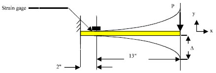 | |
| Fig. 6: | Bending of a cantilever |
The moment My for the yield point:
 |
where, “I” is the moment of inertia and c is half the thickness of the bar.
Elastic analysis: When εx = 550 με σx = Eεx = 550 10-6x200 109Pa = 110 MPa σx<σy.
As long as the normal stress σx does not exceed the yield stress σy, Hooke’s law applies and the stress distribution across the section is linear. The equation σm = Mc/I can be used to obtain the maximum value of stress.
Residual stress distribution: The distribution of the stress at the location of the strain gage due to the load is shown in Fig. 7a. The distribution of the reversed stresses due to the opposite bending moment required to unload the member is shown in Fig. 7b. Superposing the two distributions of stresses, results no residual stress since theoretically the yielding stress was not exceded.
In the case of existence of original residual stress in the bar, the original residual stress distribution is added to the other two stress distributions to give the final residual stress Fig. 8a-b.
Elastoplastic analysis (with no cyclic strain hardening): The normal strain εx varies linearly with the distance y from the neutral axis: εx = -y/c εm.
y represents the distance of a point considered from the neutral axis and εm is the maximum strain at the surface. If σm<σy, then the equation σm = Mc/I can be used as shown on Fig. 9.
 | |
| Fig. 7(a-b): | Elastically loading and unloading beam, (a) Elastically loading beam and (b) Elastically unloading the beam |
 | |
| Fig. 8(a-b): | Elastically loading the beam with pre-existing residual stress, (a) Elastically loading beam and (b) Elastically unloading the beam |
 | |
| Fig. 9: | Stress distribution in the beam before yielding occurs |
As the bending moment increases σm reaches σy Fig. 10:
| (1) |
As the bending moment increases, plastic zones develop, with the stress uniformly equal to σy (assuming ideal yield behavior) Fig. 11. In the elastic zone σx varies linearly with y according to following equation:
| (2) |
where, yy is half the thickness of the elastic core. As the bending moment increases, the plastic zones expand until the deformation is fully plastic as shown in Fig. 12:
 | |
| Fig. 10: | Stress distribution in the beam when yielding occurs |
 | |
| Fig. 11: | Stress distribution in the beam when the maximum stress exceeds yielding |
 | |
| Fig. 12: | Entire beam is plastic |
| (3) |
Or:
| (4) |
These equations were derived (Beer and Johnston, 1981) with no particular relation between stress and strain. The value of a bending moment corresponding to a given elastic core 2yy:
 | (5) |
Using Eq. 1 yields the following equation:
 | (6) |
Recall that σx is given by Eq. 2 when y is between 0 and yy and equal to -σy when y is between yy and c. My is the maximum elastic moment.
When yy approaches zero, M approaches Mp = 3/2 My for a fully plastic zone:
| • | yy when εx = 1550 με |
| • | εx = 1550 με |
| • | σx = Eεx = 1550 10-6 x200 109 Pa = 310 Mpa |
 | (7) |
My was calculated previously My = 95.877 N.m. Substituting M and My into Eq. 6:
 | (8) |
yy = 0.0034 m = 3.4 mm
Residual stress distribution: The elastic core in this case is 2yy = 6.8 mm. The distribution of the stress due to the 118.89 Nm moments is shown in Fig. 13a. Figure 13b shows the stress distribution due to the inverse load of 118.89 Nm. Superposing these two distributions gives us the final residual stress distribution in Fig. 13c.
In the case of the existence of original residual stress, the original residual stress will be added to the previous two stress distributions, Fig. 14a-b.
Analysis of the first VSR cycle with consideration of cyclic strain hardening (no preexisting residual stress): Suppose that the surface strain amplitude is 1550 με which exceeds the yielding strain (1250 με) for hot rolled steel used in the experiments. A complete cycle is analyzed with the assumption that there is no original residual stress to begin with. Also, assuming that the cyclic strain hardening effect takes place by increasing the yield stress in the second half cycle by 3%. The plastic portion of the stress strain curve is simply the value of the yield stress.
The first half cycle shown in Fig. 15a-c consists of bending the cantilever upward to obtain the required surface strain amplitude of 1550 με and then releasing the bar. The residual stress distribution from Fig. 15c is used as original residual stress in the second half cycle Fig. 16a-d. In the second half cycle it is assumed that the yield stress is increased (strain hardening) by 3%. The yield stress then is equal to 257.5 MPa. Figures 16a-d shows the final residual stress distribution after one cycle is completed.
 | |
| Fig. 13(a-c): | Residual stress distribution in the beam after unloading, (a) Loading (b) Unloading and (c) Results |
Analysis of the first VSR cycle with cyclic strain hardening and initial residual stress: Residual stresses are generated by non-uniform plastic deformation (Dieter, 1986). The general method by which residual stresses are produced in a rolling process is shown in Fig. 17a-b. In this example the rolling conditions are such that plastic flow occurs only near the surfaces of the sheet. The surface grains in the sheet are deformed and tend to elongate while the grains in the center of the sheet are unaffected. Since, the sheet must remain a continuous whole, the surface and the center regions of the sheet must undergo a strain accommodation. The center fibers tend to restrain the surface fibers from elongating while the surface fibers seek to stretch the central fibers of the sheet. The result is a residual stress pattern in the sheet which consists of a high compressive stress at the surface and a tensile residual stress at the center of the sheet Fig. 17b.
 | |
| Fig. 14(a-b): | Original stress, (a) Loading beam and (b) Unloading beam |
 | |
| Fig. 15(a-c): | First half cycle σy = 250 106 Pa yy = 3.4mm, (a) Applied stress (b) Reverse load and (c) Residual stress |
Similar to previous section the surface strain amplitude of 1550 με is used which correlates with one of the strain values used in the experiments. It is assumed that the strain hardening effect increases the yield stress in the second half cycle by 3%.
From the experimental data and from literature (Dieter, 1986) it was found that the distribution of original residual stress in the specimens used is of the form: X = -Y4+(1/8)4 Fig. 18a-d.
 | |
| Fig. 16(a-d): | Second half cycle σy = 257.5 106 Pa yy = 3.66 mm, (a) Residual stress from the first half cycle (b) Reverse load (c) Applied stress and (d) Residual stress |
| |
| Fig. 17(a-b): | Resulting distribution of residual stress over thickness of sheet, (a) Rolling and (b) Stress distribution |
| |
| Fig. 18(a-d): | Second half cycle σy = 250 106 Pa yy = 3.4 mm, (a) Original residual stress (b) Reverse load (c) Applied stress and (d) Residual stress |
| |
| Fig. 19(a-e): | Second half cycle σy = 257.5 106 Pa yy = 3.66 mm, (a) Residual stress from the first half (b) Reverse load (c) Applied stress (d) Residual stress and (e) Superimposed stresses |
This function is plotted on the XY coordinate where the thickness of the bar is represented by y and the stress magnitude is represented by x. Figure 18 and 19 show the distribution of residual stress in the first and in the second half cycle, respectively.
MODELING
Modeling is divided into two main parts: First, a study of the elastic and plastic parts of the stress strain curve to find the variation of plastic strain versus the applied strain. Second, a direct application of the Bauschinger effect is done to compare experimental and theoretical data.
Elastic zone: For a surface strain εx = 550 με, the applied stress σx = Eεx = 200 109 Pax550 10-6 = 110 Mpa, Fig. 20.
From the experimental data, the maximum residual stress observed in the bars was around 100 MPa:
| • | The total value for σx is 110 MPa+100 M |
| • | The yielding moment My = σy I/c, My = 95.877 N.m from previous calculation |
| • | Maximum moment M = σx I/c |
 | |
| Fig. 20: | Elastic zone |
where, I = 1.8263 10-9 m4 for the 1x3/8 in (25.4x9.525 mm) bar area:
| (9) |
yy is half the elastic zone (Fig. 11) and can be calculated from Eq. 6:
| (10) |
| (11) |
This means the whole bar is still elastic when loading at 550 με and no change in residual stress should be expected after unloading.
Plastic zone: Calculation of the plastic strain after unloading the first half cycle is considered for three cases (1) Assuming perfectly elastic and perfectly plastic curves, (2) Assuming that the plastic curve is a straight line of slope 0.1E and (3) Plastic curve is of the form σ = kεn.
Perfectly elastic and perfectly plastic curves: Figure 21 shows that the maximum strain is represented by the abscissa of point Q. Yielding strain is represented by the abscissa of point Y. Strain after unloading is represented by the abscissa of point P. Figure 21 shows that:
εp = OP = YQ = εQ-εY, when εQ = 1550 με and εY = 1250 με
εp = 1550-1250 = 300 με
Slope of the plastic curve is 0.1E (0.1 young’s modulus): εQ-εY = 1550-1250 = 300 με. The stress for point Q then is σQ = 0.1E (300 με)+250 = 256 MPa. From Fig. 22, point A has an abscissa εA as a projection of point A to the abscissa axis.
 | |
| Fig. 21: | Perfectly elastic perfectly plastic |
 | |
| Fig. 22: | Plastic curve is 0.1 E |
From the elastic line with slope E. σQ = EεAεA = σQ/E εA = 256 MPa/200 103 MPa = 1280 με, then εp = εQ-εA = 1550-1280 = 270 με.
Plastic curve is of the form σ = kεn: The unloading line is parallel to the elastic line. The equation of the unloading line is σ = E(ε-P) Fig. 23.
From this figure the projection of point A from the plastic line to the abscissa axis is the point εA:
εA = σQ/E and εP = εQ-εA
σy = 335 Mpa, E = 690 Mpa, εy = 1700 με
σ = kεn
 | |
| Fig. 23: | Plastic curve |
where, n and k are calculated from the plastic curve data and based on true stress true strain calculation:
n = 0.1459 and k = 99385 psi (690 MPa)
For an applied strain εa = 1850 με:
σ = kεn σQ = 690 (1850 10-6)0.1459 +335 MPa
σQ = 610 MPa
εA = σQ/EεA = 610 MPa/197067 MPa = 310 με
εP = εQ-εA = 1850-310 = 1540 με
Variation of plastic strain with the applied strain: Using the applied strain of 1550 με, the thickness of the elastic zone was calculated previously:
yy = 3.4 mm
At this particular point the stress and the strain are calculated from the elastic line of slope E as follows:
σ = Eε = My/I
ε = My/IE
σ = 200x103x1.11x10-3 = 222 MPa
The equation of the line with slope m = 0.1 E then becomes:
σ-222 = 0.1E (ε-1110) or My/I-222 = 0.1E (ε-1110)
ε = 1/0.1E (My/I-222)+1.11 10-3
Finding εQ for each value of y and calculating the plastic strain εp, the plastic strain versus the applied strain is shown in Fig. 24.
Prediction of remaining residual stress after one half strain cycle: Measured Young’s modulus E = 197067 Mpa:
Measured yield stress σy = 335 Mpa
Original residual stress at the surface σInitial = -100 Mpa is taken as an average from the experimental work.
Loading and unloading between the two strains ranges ±1550 and ±1350 με is shown in Fig. 25 and 26:
| • | The yield strain εy = (-335-(-100))/197067 = -1192 με |
| • | The straight line passing through the two points (εa; σy) and (0; σfinal) has a slope equal to E: |
 | |
| Fig. 24: | Variation of plastic strain with the applied strain |
 | |
| Fig. 25: | Bending the bar in the first half cycle, perfect plastic behavior |
 | |
| Fig. 26: | Bending the bar in the first half cycle, strain hardening effect |
(12) |
σfinal = σflow-Eεapplied
σremaining = σinitial-σfinal
where, εa = applied strain and σr = remaining stress:
| (13) |
where, σflow = σy for perfectly plastic materials. And σflow = kεn for strain hardening materials. Equation 13 is used to help explain the VSR experimental results.
CONCLUSION
This study started up with explanation of cyclic loading including stress controlled and strain controlled cyclic functions. In addition, the yielding strain and the yielding moment of a cantilever were studied to show the theoretical distribution of residual stresses in the bar after bending.
The elastic and plastic parts of the stress strain curve were analyzed to find the variation of plastic strain versus the applied strain. A direct application of the Bauschinger effect is done to compare experimental and theoretical data.
The mathematical model was derived based on the elastic and plastic parts of the stress strain curve.
Cyclic loading is capable of reducing residual stresses from the first cycle if this cycle is in the plastic zone. When the first cycle is in the elastic zone, no reduction in residual stresses was noticed. So, for stress relief to occur, a critical cyclic strain amplitude must be exceeded.
Further work on vibratory stress relief will include using the model in later work to help explain the vibratory stress relief experimental results.
REFERENCES
- Qinghua, L., C. Ligong and N. Chunzhen, 2008. Effect of vibratory weld conditioning on welded valve properties. Mech. Mater., 40: 565-574.
CrossRefDirect Link - Rao, D., D. Wang, L. Chen and C. Ni, 2007. The effectiveness evaluation of 314L stainless steel vibratory stress relief by dynamic stress. Int. J. Fatigue, 29: 192-196.
CrossRefDirect Link - Sun, M.C., Y.H. Sun and R.K. Wang, 2004. The vibratory stress relief of a marine shafting of 35# bar steel. Mater. Lett., 58: 299-303.
CrossRefDirect Link - Sun, M.C., Y.H. Sun and R.K. Wang, 2004. Vibratory stress relieving of welded sheet steels of low alloy high strength steel. Mat. Lett., 58: 1396-1399.
CrossRefDirect Link - Tuegel, E.J. and C.L. Brooks, 1997. Cyclic relaxation in compression-dominated structures. Int. J. Fatigue, 19: 245-251.
CrossRefDirect Link - Xu, J., L. Chen and C. Ni, 2007. Effect of vibratory weld conditioning on the residual stresses and distortion in multipass girth-butt welded pipes. Int. J. Pressure Vessels Piping, 84: 298-303.
CrossRefDirect Link - Zhao, X.C., Y.D. Zhang, H.W. Zhang and Q. Wu, 2008. Simulation of vibration stress relief after welding based on FEM. Acta Metallurgica Sinica (English Lett.), 21: 289-294.
CrossRefDirect Link